FRI and Proximity Proofs, Part 1 — Reed-Solomon Codes, IOPs of Proximity, Quotienting and Folding
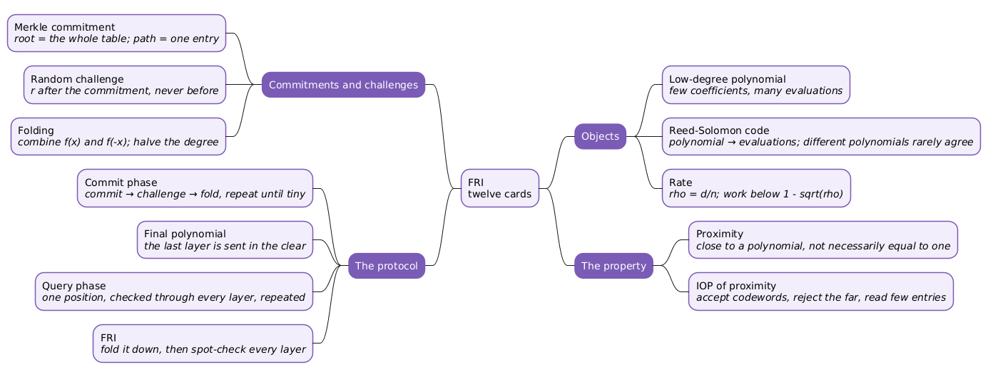
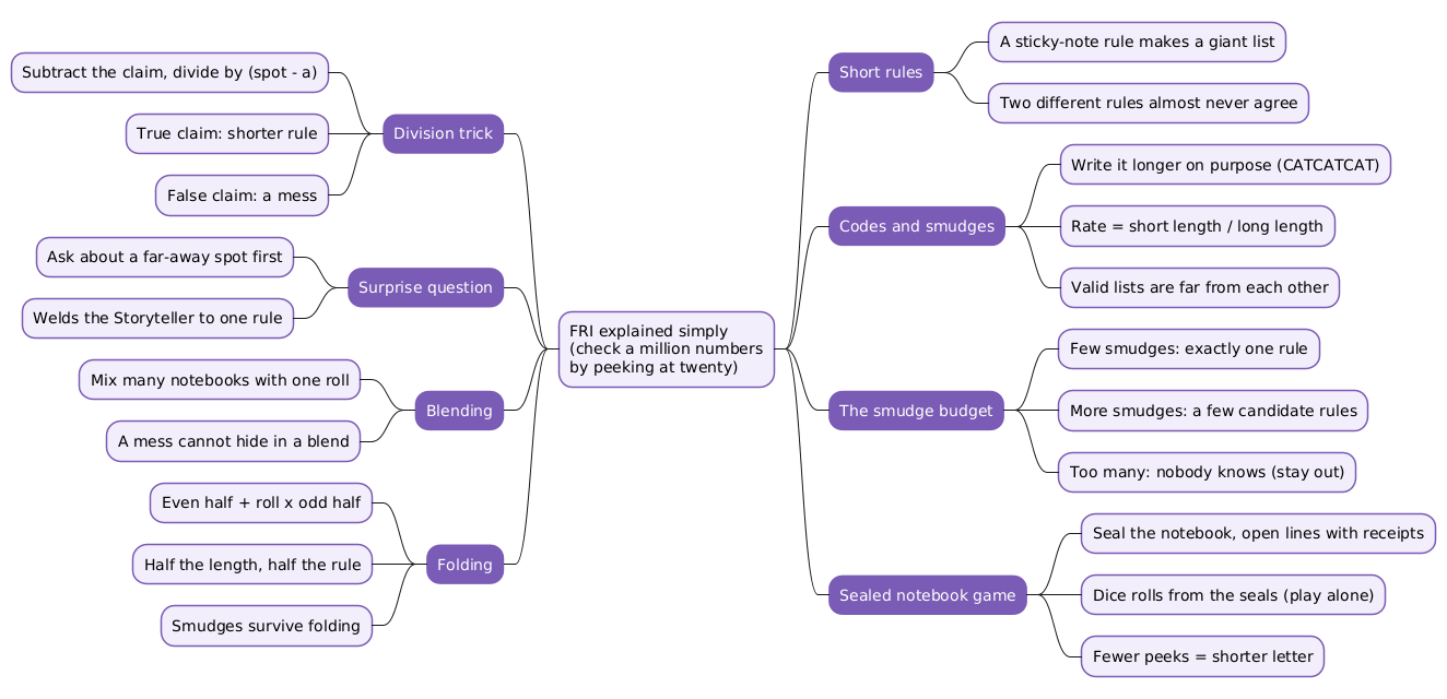
FRI stands for Fast Reed-Solomon Interactive Oracle Proof of Proximity. Fix a finite field \(\mathbb F\), a subset \(L \subseteq \mathbb F\) and a function \(y : L \to \mathbb F\) that the prover has committed to. FRI lets the prover convince a verifier, who reads only a handful of positions of \(y\), that \(y\) is close to a Reed-Solomon codeword, in other words close to the evaluation table of some polynomial of bounded degree. That statement is modest on its own. Its value comes from what can be built on top of it: a polynomial commitment scheme with no trusted setup and no elliptic curves, and from there a hash-based SNARK.
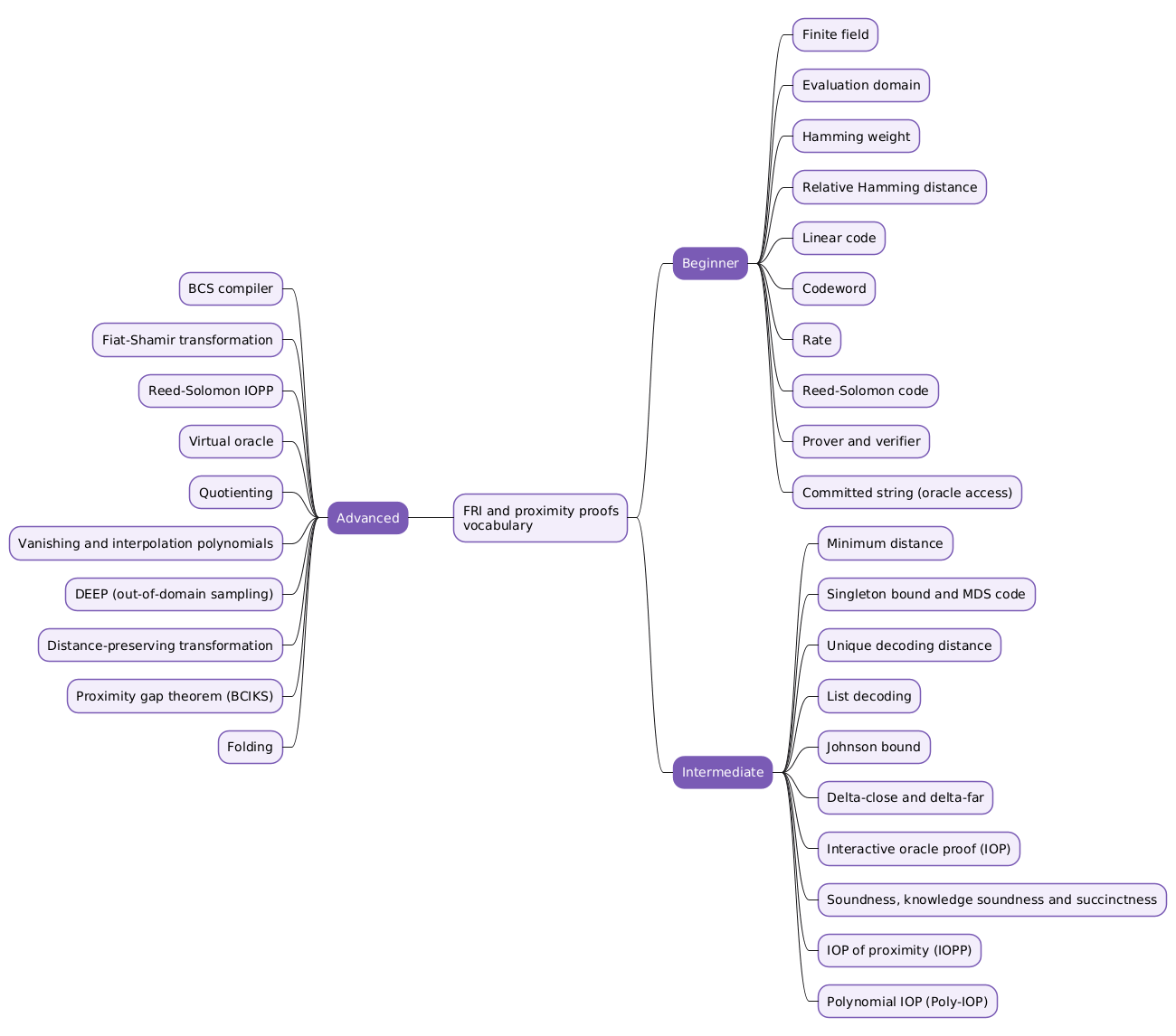
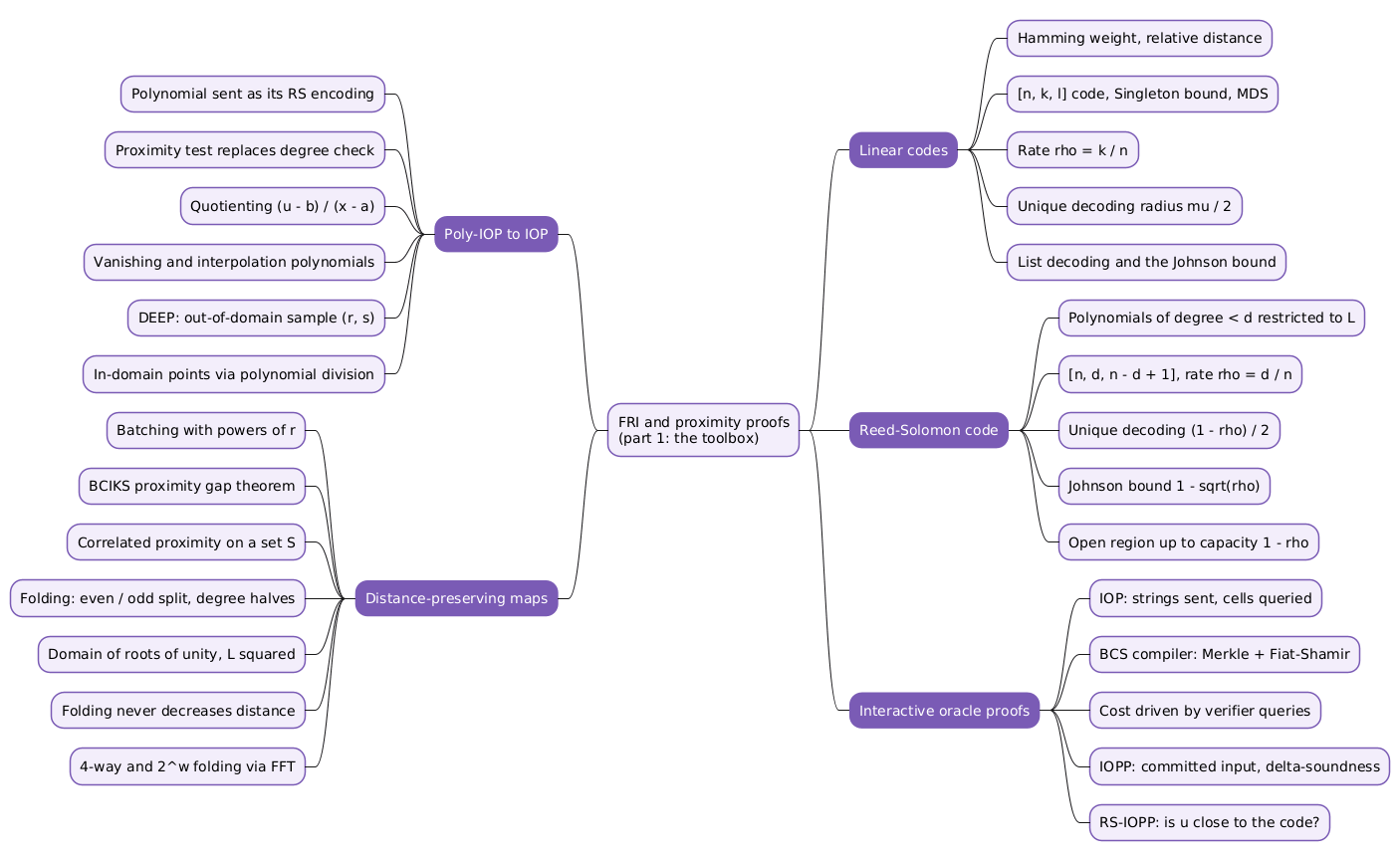
This article is based on a ZK Whiteboard Sessions lecture by Dan Boneh, the first half of a two-part module on FRI and proximity proofs. It covers everything the construction of FRI depends on but stops short of FRI itself: linear codes and list decoding, the Reed-Solomon code and its Johnson bound, interactive oracle proofs and the BCS compiler, the quotienting trick that turns a proximity test into an evaluation proof, and the two distance-preserving transformations (batching and folding) on which the FRI protocol rests. Part 2, when it is written, will assemble these pieces into FRI and its successors.
The notation follows the slides so that they remain usable alongside the text. Where a fact is stated without proof here, the reference list points to the paper that carries the argument.
This article has been made with the help of Claude Code and several custom skills
What FRI proves, and why anyone cares
The setting is a prime field \(\mathbb F = \{0, 1, \dots, p-1\}\) with arithmetic modulo \(p\), an evaluation domain \(L \subseteq \mathbb F\) of size \(n\), and a committed function \(y : L \to \mathbb F\). “Committed” means the verifier holds a commitment to \(y\) and can ask for the value of \(y\) at individual points, paying for each request. FRI is a protocol in which the prover proves that \(y\) is close, in Hamming distance, to some Reed-Solomon codeword, while the verifier opens only a small number of positions.
Two questions follow immediately. What is a Reed-Solomon codeword, and what does “close” mean precisely? And why would a proof system need such a statement? The first question needs a short course in coding theory, which is the next section. The second is answered in the section on compiling a Poly-IOP: a proximity proof is exactly the missing piece that lets a verifier who can only read cells of a string treat that string as if it were a polynomial.
The research this rests on splits into two families. One builds SNARKs on Reed-Solomon codes: FRI, DEEP-FRI, the proximity-gap theorem, STIR. The other replaces Reed-Solomon with codes that encode faster or work over any field. Part 1 stays with Reed-Solomon; the other family is where current research is concentrating, and it is the subject of the second half of the module.
A crash course in linear codes
Hamming weight and relative distance
For a vector \(u \in \mathbb F^n\), the Hamming weight \(\lVert u \rVert_0\) is the number of non-zero coordinates. A compact way to write it is
[\begin{aligned} \lVert u \rVert_0 = \sum_{i=1}^{n} u_i^{\,0}, \qquad \text{with the convention } 0^0 = 0, \end{aligned}]
so that every non-zero coordinate contributes \(1\) and every zero coordinate contributes \(0\). This is a norm, the zero norm, and it satisfies the triangle inequality like any other norm.
The relative Hamming distance between two vectors normalises the number of disagreeing coordinates by the length:
[\begin{aligned} \Delta(u, v) = \frac{\lVert u - v \rVert_0}{n} \in [0, 1]. \end{aligned}]
Two words of length \(5\) that differ in \(3\) positions are at relative distance \(3/5\).
Linear codes, the Singleton bound and MDS codes
A linear code \(C\) with parameters \([n, k, \ell]\) over \(\mathbb F\) is a linear subspace of \(\mathbb F^n\) of dimension \(k\) in which every non-zero codeword has Hamming weight at least \(\ell\). The three parameters recur throughout:
- \(n\), the length of a codeword;
- \(k\), the dimension of the subspace, so the code holds \(p^k\) codewords;
- \(\ell\), the minimum Hamming weight, with \(\mu = \ell / n\) the relative minimum distance.
Two facts follow directly. First, any two distinct codewords \(u, v \in C\) satisfy \(\Delta(u, v) \ge \mu\): their difference \(u - v\) is itself a non-zero codeword, so it has weight at least \(\ell\). Second, the Singleton bound: \(k \le n - \ell + 1\). The proof is one line. Delete the first \(\ell - 1\) coordinates of every codeword. Two codewords that agreed on the remaining \(n - \ell + 1\) coordinates would differ in fewer than \(\ell\) positions, which is impossible, so the truncated words are all distinct and there are at most \(p^{\,n-\ell+1}\) of them.
A code that meets the Singleton bound with equality, \(k = n - \ell + 1\), is as large as a code with that minimum distance can be. Such codes are called Maximum Distance Separable, or MDS. The Reed-Solomon code is the classic example.
Encoding and rate
Since \(C\) is a subspace of dimension \(k\), it has a basis \(c_1, \dots, c_k\). A message \(m \in \mathbb F^k\) is encoded as the linear combination \(\sum_i m_i c_i\), so encoding is a linear map \(\mathbb F^k \to \mathbb F^n\) that stretches a \(k\)-symbol message into an \(n\)-symbol codeword. The rate
[\begin{aligned} \rho = \frac{k}{n} \in (0, 1] \end{aligned}]
measures that stretch: \(1/\rho\) is the expansion factor. A higher rate means less expansion and a faster encoder, which is why code-based SNARKs would like \(\rho\) to be large; in practice a rate of \(1/2\), a codeword twice the size of the message, is a common compromise. The worked example later in this article uses \(\rho = 1/4\).
Unique decoding
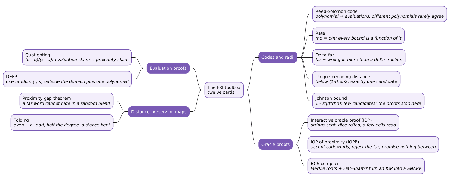
Take two distinct codewords \(u, v\) and an arbitrary word \(w \in \mathbb F^n\) that is not necessarily in the code. If both \(u\) and \(v\) were within relative distance \(\mu/2\) of \(w\), the triangle inequality would give \(\Delta(u, v) \lt \mu\), contradicting the minimum distance. So a Hamming ball of radius \(\mu/2\) around any word contains at most one codeword. The radius \(\mu / 2\) is called the unique decoding distance.
Most words are not uniquely decodable. The set of uniquely decodable words is the union, over all codewords, of a ball of radius \(\ell/2\). A ball of that radius holds about \(\binom{n}{\ell/2}\, p^{\ell/2}\) words (choose which \(\ell/2\) coordinates to change, then choose their new values), and the Singleton bound caps the number of codewords at \(p^{\,n-\ell+1}\). The product is far smaller than \(p^n\), so almost every word in \(\mathbb F^n\) lies outside every unique-decoding ball.
List decoding and the Johnson bound
That observation motivates list decoding. For a word \(w\), a code \(C\) and a radius \(\delta \in [0, 1]\), define
[\begin{aligned} \mathrm{List}(w, C, \delta) = {\, c \in C : \Delta(w, c) \le \delta \,}. \end{aligned}]
For \(\delta \lt \mu/2\) the list has at most one element, by the argument above. The question is how the list grows past that radius, and the answer has four regimes:
| Radius \(\delta\) | Size of \(\mathrm{List}(w, C, \delta)\) |
|---|---|
| \(0 \le \delta \lt \mu/2\) (unique decoding) | at most \(1\) |
| \(\mu/2 \le \delta \lt J(\mu)\) (up to the Johnson bound) | at most \(1/\varepsilon_\delta\), a quantity that grows to infinity as \(\delta \to J(\mu)\) |
| \(J(\mu) \le \delta \lt \mu\) (up to the capacity bound) | unknown in general; depends on the code |
| \(\delta \ge \mu\) (above capacity) | exponentially large; at \(\delta = 1\) the list is the whole code |
The Johnson bound \(J(\mu)\) is a function of the minimum distance alone; it always exceeds the unique decoding distance, and below it the list size is bounded by an explicit expression \(1/\varepsilon_\delta\) whose denominator tends to zero at the bound itself. The proof is about half a page and is a reasonable exercise. Everything in this article and in FRI’s analysis relies on proven bounds, so \(\delta\) is always kept below the Johnson bound.
Two pieces of vocabulary close the section. A word \(w\) is \(\delta\)-close to \(C\) if some codeword lies within relative distance \(\delta\) of it, written \(\Delta(w, C) \le \delta\); it is \(\delta\)-far if every codeword is at distance greater than \(\delta\), written \(\Delta(w, C) \gt \delta\).
The Reed-Solomon code
Polynomials as codewords
Let \(\mathbb F^{\lt d}\) denote the polynomials over \(\mathbb F\) of degree less than \(d\). It is a linear space of dimension \(d\), one dimension per coefficient from the constant term to the coefficient of \(x^{d-1}\). A polynomial \(f\) defines a function on the whole field, but the code only looks at it on the domain \(L\): write \(\bar f\) for the restriction of \(f\) to \(L\).
| A function from \(L\) to \(\mathbb F\) is the same object as a vector of length $$n = | L | \(, once the elements of\)L$$ are put in a fixed order: list the values at every point of the domain. This article moves freely between the two views. |
The Reed-Solomon code with field \(\mathbb F\), evaluation domain \(L\) and degree bound \(d \lt n\) is
[\begin{aligned} \mathrm{RS}[\mathbb F, L, d] = {\, \bar f : f \in \mathbb F^{\lt d} \,}. \end{aligned}]
Its codewords are the evaluation tables of low-degree polynomials. A non-zero polynomial of degree at most \(d - 1\) has at most \(d - 1\) roots, so every non-zero codeword has at least \(n - d + 1\) non-zero entries. The code is therefore an \([n, d, n - d + 1]\) linear code; it meets the Singleton bound with equality, so it is MDS, and it contains \(p^d\) codewords, one per polynomial. Its rate is \(\rho = d / n\).
Encoding a message is concrete: treat the \(d\) message symbols as the coefficients of a polynomial and evaluate it on \(L\). At rate \(1/2\), a polynomial of degree less than \(d\) is evaluated at \(2d\) points.
The list-decoding picture in terms of the rate
For Reed-Solomon codes it is more convenient to express everything in terms of \(\rho\) rather than \(\mu\), and to write \(\mathrm{List}(w, d, \delta)\) for the list of codewords of \(\mathrm{RS}[\mathbb F, L, d]\) within distance \(\delta\) of \(w\), since the degree determines the code. Substituting \(\ell = n - d + 1\) and \(\rho = d/n\):
- the unique decoding distance \(\mu / 2\) becomes approximately \((1 - \rho)/2\);
-
the Johnson bound becomes \(1 - \sqrt{\rho}\), below which $$ \mathrm{List}(w, d, \delta) \le 1/\varepsilon_\delta$$; - the capacity bound \(\mu\) becomes approximately \(1 - \rho\).
Between \(1 - \sqrt\rho\) and \(1 - \rho\) the behaviour of Reed-Solomon list sizes is an open problem. There is a conjecture that the list stays polynomial in \(n\) throughout that interval. A 2024 result proves the conjecture when the evaluation domain \(L\) is chosen at random. FRI uses a highly structured domain, a group of roots of unity, and for structured domains the question remains open.
Plugging in \(\rho = 1/4\), so that codewords are four times the size of the message: the unique decoding distance is \(3/8\) and the Johnson bound is \(1/2\). From \(0\) to \(1/2\) the list size is under control; above \(1/2\) nothing is proven. The SNARKs built later get more efficient as \(\delta\) grows, so there is pressure to push \(\delta\) up, and the Johnson bound is where the proven guarantees end.
Interactive oracle proofs
The IOP model
An interactive oracle proof is an information-theoretic object: it lets a proof system be designed and analysed without any cryptographic assumption, with the cryptography added afterwards by a compiler. Fix a relation \(R\) of pairs \((x, w)\), where \(x\) is the instance and \(w\) the witness; the only requirement is that membership in \(R\) is decidable in polynomial time. A hash preimage relation, \(x = H(w)\), or a commitment-opening relation are typical examples.
An IOP for \(R\) is a pair of algorithms. The prover \(P\) receives \((x, w)\); the verifier receives \(x\) only. They interact in rounds: the prover sends a string \(\pi_0\), the verifier answers with a random challenge \(\alpha_1\), the prover sends \(\pi_1\), and so on until the prover sends its last string \(\pi_k\). Then the verifier runs a decision algorithm \(V\) that takes \(x\) and all the challenges as explicit input, and gets the strings \(\pi_0, \dots, \pi_k\) as oracles: it may ask for the third cell of \(\pi_0\) or the fifth cell of \(\pi_1\), as many cells as it wants, and outputs accept or reject based on what it read.
Four properties define a useful IOP:
- Completeness. When \(V\) interacts with the honest prover on \((x, w) \in R\), it always accepts.
- Soundness. For every prover \(P^\star\) and every \(x\) that has no witness at all, \(V\) accepts with negligible probability, taken here to mean at most \(2^{-128}\).
- Knowledge soundness. If a prover convinces \(V\) to accept \(x\), then that prover knows a \(w\) with \((x, w) \in R\). The formal definition is left to the papers.
- Succinctness. The verifier’s running time must be far smaller than the time needed to evaluate \(R\) directly.
Without the fourth property there is a trivial protocol: send the witness and let the verifier check it. Succinctness rules that out, and it has a concrete consequence for the design: since reading a cell costs time, a succinct verifier makes very few oracle queries. Most of the design effort in code-based SNARKs goes into keeping that query count down.
From an IOP to a SNARK: the BCS compiler
An IOP for \(R\) yields a SNARK for \(R\) through the BCS compiler, named after Ben-Sasson, Chiesa and Spooner. It works in two steps.
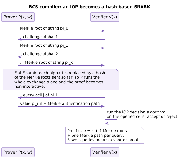
In the first step, the prover sends a Merkle commitment to each string \(\pi_i\) instead of the string itself. Whenever \(V\) queries cell \(j\) of \(\pi_i\), the prover answers with the value and a Merkle proof for that cell. Nothing else changes. The result is an ordinary interactive proof, with no oracles, whose security now rests on the collision resistance of the Merkle hash function rather than being unconditional.
In the second step the Fiat-Shamir transformation removes the interaction. The prover derives each challenge by hashing the Merkle commitments sent so far, then runs the verifier itself and appends a Merkle proof for every cell the verifier asks for. The whole SNARK proof is the list of commitments plus the Merkle proofs at the queried positions, and the SNARK verifier replays the decision algorithm to confirm it accepts. A theorem states that if the IOP has a property called round-by-round soundness, the compiled system is a SNARG, or a SNARK when the IOP is knowledge sound. Chiesa and Yogev’s book Building Cryptographic Proofs from Hash Functions is devoted to the precise definitions and to the proof that this transformation is secure.
The efficiency of the result is easy to read off. The prover’s main cost is Merkle-committing to every string it sends, so shorter strings mean a faster prover. The proof size has one commitment per string and one Merkle proof per verifier query, and since a Merkle proof is a full authentication path, the query count dominates. Reducing verifier queries is the central optimisation target.
IOPs of proximity
An IOP of proximity, or IOPP, generalises the IOP in one respect: the relation now has triples \((x, y, w)\), where the instance is the pair \((x, y)\) and \(y\) is itself one of the strings the prover could have sent. The prover receives \(y\) in full; the verifier receives \(x\) explicitly but gets \(y\) only as an oracle, and can read cells of it exactly as it reads cells of \(\pi_0, \dots, \pi_k\). An IOPP is therefore a way to prove properties of a committed string.
Soundness is relaxed to match. Say that \((x, y)\) is \(\delta\)-far from \(R\) if for every \(y'\) within relative distance \(\delta\) of \(y\) and every \(w\), the triple \((x, y', w)\) is not in \(R\). Then:
- Completeness is unchanged: an honest prover on \((x, y, w) \in R\) is always accepted.
- \(\delta\)-soundness requires that whenever \((x, y)\) is \(\delta\)-far from \(R\), the verifier accepts with negligible probability.
- When \((x, y)\) is neither in the relation nor \(\delta\)-far from it, the verifier may do anything; no guarantee is required.
The IOPP that matters here is the Reed-Solomon IOPP. Its instance is the code \(C = \mathrm{RS}[\mathbb F, L, d]\), its committed word is an arbitrary function \(u : L \to \mathbb F\), and the relation holds when \(u \in C\). A \(\delta\)-sound Reed-Solomon IOPP therefore accepts every codeword and rejects, with overwhelming probability, every word whose distance from the code exceeds \(\delta\). FRI is one efficient protocol of this kind.
From a Poly-IOP to an IOP
Poly-IOPs and the two compilation routes
A Poly-IOP is an IOP in which the strings the prover sends are constrained to be polynomials of bounded degree, and the verifier, instead of reading cells, may evaluate any of those polynomials at any point of \(\mathbb F\). Completeness and soundness are defined as for IOPs. Most deployed SNARKs are Poly-IOPs compiled down: the standard route replaces each polynomial with a polynomial commitment and each evaluation query with an evaluation proof, producing an interactive proof, and then applies Fiat-Shamir. A previous article on this site, KZG Polynomial Commitments — The Terms and Formulas, From Beginner to Advanced, covers the pairing-based instantiation of that route. Poly-IOPs over univariate polynomials, such as Plonk, and over multilinear polynomials, such as HyperPlonk, both exist; SNARKs derived from multilinear Poly-IOPs have turned out to be more efficient, and the field is moving in that direction, but this module stays with the univariate case.
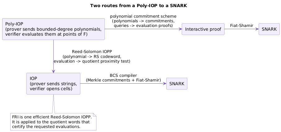
The second route is the one a Reed-Solomon IOPP opens. Convert the Poly-IOP into a plain IOP, then hand the IOP to the BCS compiler. The interesting step is the first one: the Poly-IOP world has a polynomial evaluation oracle and the IOP world has only a cell lookup oracle, so an evaluation oracle has to be simulated using cell lookups.
Representing a polynomial as a string
The natural representation is the Reed-Solomon encoding. Fix a domain \(L = \{a_1, \dots, a_n\}\). Where the Poly-IOP prover would send \(f \in \mathbb F^{\lt d}\), the IOP prover sends the string \(\pi = \bar f\), the evaluations of \(f\) at every point of \(L\), which is a codeword of \(\mathrm{RS}[\mathbb F, L, d]\). The string is treated as a function \(\pi : L \to \mathbb F\) in what follows. Nothing forces the choice of Reed-Solomon; other linear codes can encode polynomials too, sometimes faster, and that is where much current research sits.
The encoding creates an immediate problem. In the Poly-IOP the prover could only send bounded-degree polynomials; in the IOP it can send any string, including one that is not a codeword and so represents no polynomial. The verifier cannot check codeword membership by reading a few cells: a string that equals a codeword everywhere except one position is not a codeword, and the chance of opening exactly that position is negligible.
What the verifier can do is run a Reed-Solomon IOPP to check that \(\pi\) is \(\delta\)-close to the code. If the test passes, \(\pi\) is within \(\delta\) of some codeword with high probability, and if \(\delta\) is below the unique decoding distance, that codeword, and hence the polynomial it encodes, is unique. This binds the prover to a polynomial. It is not yet a polynomial commitment scheme, because there is no way to prove what that polynomial evaluates to at a point of the verifier’s choosing. Quotienting supplies that.
Quotienting
The quotient of a function by a point
Fix \(a, b \in \mathbb F\) with \(a \notin L\), and a function \(u : L \to \mathbb F\). Define the quotient function
[\begin{aligned} q(x) = \frac{u(x) - b}{x - a}, \qquad x \in L. \end{aligned}]
Because \(a\) is outside the domain, the denominator never vanishes and \(q\) is a well-defined function from \(L\) to \(\mathbb F\). Two facts about it carry the whole construction.
Fact 1. If \(u = \bar f\) for some \(f \in \mathbb F^{\lt d}\) and \(b = f(a)\), then \(q\) is a codeword of \(\mathrm{RS}[\mathbb F, L, d-1]\). The polynomial \(f(x) - b\) has \(a\) as a root, so \(x - a\) divides it and the quotient is a polynomial of degree less than \(d - 1\); \(q\) is that polynomial’s restriction to \(L\).
Fact 2. If every polynomial \(g \in \mathrm{List}(u, d, \delta)\) satisfies \(g(a) \ne b\), then \(q\) is \(\delta\)-far from \(\mathrm{RS}[\mathbb F, L, d-1]\). The proof is by contradiction: were \(q\) within distance \(\delta\) of a codeword \(\bar h\) of degree less than \(d-1\), the polynomial \(g(x) = (x-a)\,h(x) + b\) would be a degree-\(d\) polynomial with \(g(a) = b\) whose restriction agrees with \(u\) wherever \(q\) agrees with \(\bar h\), placing \(g\) in the list and violating the hypothesis.
Together: a correct claimed evaluation turns the quotient into a codeword, and a claimed evaluation that is wrong for every polynomial near \(u\) turns the quotient into a word far from the code. A Reed-Solomon IOPP run on \(q\) therefore tests whether \(b = f(a)\).
Quotienting by several points
The same idea extends to \(k\) evaluation points \(a_1, \dots, a_k \notin L\) with claimed values \(b_1, \dots, b_k\). Define the vanishing polynomial and the interpolation polynomial
[\begin{aligned} V(x) = \prod_{i=1}^{k} (x - a_i), \qquad I(a_i) = b_i \ \text{for all } i, \end{aligned}]
both of degree at most \(k\), and the quotient
[\begin{aligned} q(x) = \frac{u(x) - I(x)}{V(x)}, \qquad x \in L. \end{aligned}]
It is well defined because no \(a_i\) lies in \(L\), and the two facts carry over. If \(u = \bar f\) and \(b_i = f(a_i)\) for all \(i\), then \(q \in \mathrm{RS}[\mathbb F, L, d-k]\). If every \(g \in \mathrm{List}(u, d, \delta)\) violates at least one of the claimed evaluations, then \(q\) is \(\delta\)-far from \(\mathrm{RS}[\mathbb F, L, d-k]\). The STIR paper spells the proof out.
A first compiler, and why it is not yet sound
The pieces assemble as follows. Where the Poly-IOP prover sends \(f\), the IOP prover sends \(\pi = \bar f\). Where the Poly-IOP verifier queries \(f(a_1)\) and receives \(b_1\), the IOP parties run a Reed-Solomon IOPP to show that \(q_1 = (\pi - b_1)/(x - a_1)\) is \(\delta\)-close to \(\mathrm{RS}[\mathbb F, L, d-1]\), for a \(\delta\) fixed later. The honest prover sent a codeword, so its quotient is a codeword and the IOPP accepts; a prover whose \(b_1\) is wrong for every polynomial near \(\pi\) produces a far quotient, and the IOPP rejects.
Note that \(q_1\) is never sent. Every time the IOPP verifier wants a cell of \(q_1\), both parties compute it from the corresponding cell of \(\pi\) by one subtraction and one division. An oracle derived this way from another oracle is called a virtual oracle.
A second query \(a_2\) with answer \(b_2\) is handled the same way with \(q_2\). After both IOPPs accept, the verifier knows that there exist polynomials \(f_1, f_2 \in \mathrm{List}(\pi, d, \delta)\) with \(f_1(a_1) = b_1\) and \(f_2(a_2) = b_2\). The defect is that \(f_1\) and \(f_2\) need not be the same polynomial. When \(\delta\) exceeds the unique decoding distance the list can hold several polynomials, and a malicious prover may answer each query from whichever list member is convenient. In the Poly-IOP, sending \(f\) committed the prover to one polynomial; in this compilation it does not, so the compilation is invalid as it stands.
DEEP: one out-of-domain sample fixes it
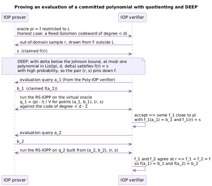
The fix, called DEEP for Domain Extension for Eliminating Pretenders, costs a single extra exchange. Before any evaluation query, the verifier samples a random \(r \in \mathbb F \setminus L\), an out-of-domain sample, and the prover replies with a value \(s\) that is meant to be \(f(r)\). The claim is that the pair \((r, s)\) commits the prover to one polynomial in the list.
| Call it a bad event if two distinct polynomials \(f_1, f_2 \in \mathrm{List}(\pi, d, \delta)\) both evaluate to \(s\) at \(r\). Two distinct polynomials of degree less than \(d\) agree on fewer than \(d\) points, otherwise their difference would have too many roots, so for a fixed pair the probability that a uniformly random \(r\) lands on one of those agreement points is at most $$d / ( | \mathbb F | - | L | )$$. A union bound over all pairs in the list gives |
[\begin{aligned} \Pr[\text{bad event}] \le |\mathrm{List}(\pi, d, \delta)|^2 \cdot \frac{d}{|\mathbb F| - |L|}. \end{aligned}]
This is where the Johnson bound enters. For \(\delta \lt 1 - \sqrt\rho\) the list size is bounded and small, so when the field is large enough the denominator dominates and the bad event is negligible. When the field is too small for that, the verifier samples several values \(r\) instead of one, and the same argument goes through. Either way, once the prover has answered \(s\), with high probability exactly one polynomial in the list satisfies \(f(r) = s\), and that is the polynomial the prover is now bound to.
The full compiler then handles each evaluation query with a two-point quotient. For query \(a_1\) with answer \(b_1\), the parties run a Reed-Solomon IOPP showing that the quotient of \(\pi\) by the points \((a_1, b_1)\) and \((r, s)\) is \(\delta\)-close to \(\mathrm{RS}[\mathbb F, L, d-2]\). Acceptance implies some \(f_1\) close to \(\pi\) with \(f_1(a_1) = b_1\) and \(f_1(r) = s\). Query \(a_2\) is handled identically, still using the same \((r, s)\), and yields an \(f_2\) with \(f_2(a_2) = b_2\) and \(f_2(r) = s\). Since \(f_1\) and \(f_2\) both lie in the list and agree at \(r\), they are equal with high probability. The verifier has learned what it needed: a single polynomial \(f\), committed to by the prover, with \(f(a_1) = b_1\) and \(f(a_2) = b_2\).
Two remarks on the compiler
Evaluation points inside the domain. Everything above assumed the evaluation point lies outside \(L\), because the quotient divides by \(x - a\) and would divide by zero at \(x = a\). If the Poly-IOP verifier wants \(f(a)\) for some \(a \in L\), the remedy is to view the quotient as a polynomial rather than a function. When \(f(a) = b\) and \(f(r) = s\), the denominator \((x-a)(x-r)\) divides the numerator \(f(x) - I(x)\) exactly, so the quotient is a polynomial of degree less than \(d - 2\), and \(q(a)\) is simply that polynomial evaluated at \(a\). From the honest prover’s side, \(q\) is just the Reed-Solomon encoding of the quotient polynomial, and the technique covers in-domain points as well.
Cost. As described, the compiler runs one Reed-Solomon IOPP per evaluation query, and each IOPP is expensive. The way out is to batch many proximity claims into one, and that requires the tools of the next section.
Distance-preserving transformations
A distance-preserving transformation takes functions \(u_1, \dots, u_k\) over a domain \(L\) and a random value \(r\), and outputs a single function \(u\) over a domain \(L'\) that may differ from \(L\). It must satisfy two conditions. If every \(u_j\) is a codeword of a Reed-Solomon code, then \(u\) is a codeword of some other Reed-Solomon code, possibly with a different domain and degree, for every choice of \(r\). If even one \(u_j\) is \(\delta\)-far from the code, then \(u\) is \(\delta\)-far from the target code with high probability over \(r\). Close inputs give a close output; a single far input gives a far output. Two examples are needed for FRI.
Batching, and the proximity gap theorem
Suppose the prover has committed to words \(u_0, \dots, u_k\) and wants to show that all of them are \(\delta\)-close to \(\mathrm{RS}[\mathbb F, L, d]\). Running \(k + 1\) separate IOPPs is the naive approach. Instead, the verifier samples \(r \in \mathbb F\) and the parties form the batched word
[\begin{aligned} u^{(r)} = \sum_{j=0}^{k} r^{\,j} \, u_j, \end{aligned}]
another function from \(L\) to \(\mathbb F\), and run the IOPP once on it. The batched word is a virtual oracle: to open \(u^{(r)}\) at a cell, the prover opens every \(u_j\) at that cell and the verifier takes the linear combination itself.
The honest direction is immediate. Reed-Solomon codes are linear, so a linear combination of codewords is a codeword, for every \(r\). The other direction is a real question about polynomials: if one \(u_j\) is far from the code, why should the combination be far for almost every \(r\)? The answer took time to establish and is the proximity gap theorem of Ben-Sasson, Carmon, Ishai, Kopparty and Saraf, proven in 2020 and referred to as BCIKS. For \(\delta\) below the Johnson bound it states: if \(u^{(r)}\) is \(\delta\)-close to the code for more than an \(\mathrm{err}\) fraction of the values \(r\), then every \(u_j\) is \(\delta\)-close to the code. The quantity \(\mathrm{err}\) is explicit in the paper; in outline, it grows linearly in \(n\) when \(\delta\) is below the unique decoding distance and quadratically in \(n\) between the unique decoding distance and the Johnson bound, divided in both cases by the field size. As with DEEP, the field is assumed large enough for \(\mathrm{err}\) to be negligible, and if it is not, several values of \(r\) are used and each combination is tested. The contrapositive is the statement needed for batching: if any \(u_j\) is \(\delta\)-far, then \(u^{(r)}\) is \(\delta\)-far with high probability over \(r\).
| The theorem says more than that, and the extra is used later. Not only is each \(u_j\) \(\delta\)-close to a codeword; there is a single set \(S \subseteq L\) of size at least $$(1 - \delta)\, | L | \(such that every\)u_j\(agrees with its nearest codeword on all of\)S$$. The words are close on the same positions. This is called correlated proximity. |
The name “proximity gap” comes from what correlated proximity implies. If all the \(u_j\) match codewords on \(S\), then by linearity every combination \(u^{(r)}\) matches a codeword on \(S\) too, for every \(r\). So the fraction of values \(r\) for which \(u^{(r)}\) is \(\delta\)-close is either negligible or equal to one; nothing in between is possible. That dichotomy is the gap, and it is the single most used tool in hash-based proof systems.
Folding
| The second example is folding, the operation FRI iterates. From here on the domain is structured: \(n\) is a power of two and \(L\) is the set of \(n\)-th roots of unity in \(\mathbb F\), generated by a primitive root \(\omega\). This requires \(n\) to divide $$ | \mathbb F | - 1$$, which restricts FRI to fields with that property; IOPPs for other codes, covered in Part 2, remove the restriction. |
| Two properties of this domain matter. First, since \(n\) is even, \(\omega^{n/2} = -1\), so \(x \in L\) implies \(-x \in L\) and the domain splits into pairs \(\{x, -x\}\). Second, define \(L^2 = \{x^2 : x \in L\}\). Squaring sends both \(x\) and \(-x\) to \(x^2\), so it is a two-to-one map and $$ | L^2 | = n/2\(. Likewise\)L^4\(, the set of fourth powers, has\)n/4$$ elements, and so on. |
Folding is easiest to see on a polynomial. Take a degree-\(5\) polynomial with six coefficients and split it into an even part, holding the coefficients of \(x^0, x^2, x^4\), and an odd part, holding those of \(x^1, x^3, x^5\). Both parts are quadratic, and
[\begin{aligned} f(x) = f_e(x^2) + x \, f_o(x^2). \end{aligned}]
The folding of \(f\) with respect to a random \(r \in \mathbb F\) is the combination \(f_e + r\,f_o\), a quadratic: a polynomial of degree bound \(6\) became one of degree bound \(3\). In general, for \(f\) of degree less than \(d\), the two parts can be extracted by evaluating at \(x\) and \(-x\):
[\begin{aligned} f_e(x^2) = \frac{f(x) + f(-x)}{2}, \qquad f_o(x^2) = \frac{f(x) - f(-x)}{2x}, \end{aligned}]
since the odd monomials cancel in the sum and the even monomials cancel in the difference. The fold \(f_e + r f_o\) has degree less than \(d/2\). Two consequences follow. Given \(f(a)\) and \(f(-a)\), the fold can be evaluated at \(a^2\) with two additions and two divisions. And if \(\bar f\) is a codeword of \(\mathrm{RS}[\mathbb F, L, d]\), its fold is a codeword of \(\mathrm{RS}[\mathbb F, L^2, d/2]\): half the degree over half the domain, so the rate \(\rho\) is unchanged.
The same formulas apply to an arbitrary function \(u : L \to \mathbb F\), which is the case the protocol has to handle. Define \(u_e\), \(u_o\) and \(u_{\mathrm{fold}}\) on \(L^2\) by the relations above, using \(u(a)\) and \(u(-a)\) in place of \(f(a)\) and \(f(-a)\).
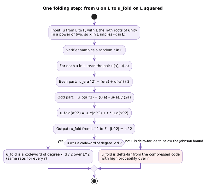
The distance-preservation lemma for folding, valid for \(\delta\) below the Johnson bound, has two halves. If \(u\) is a codeword, then \(u_{\mathrm{fold}}\) is a codeword of the compressed code \(\mathrm{RS}[\mathbb F, L^2, d/2]\) for every \(r\); this is the calculation above. If \(u\) is \(\delta\)-far from \(\mathrm{RS}[\mathbb F, L, d]\), then \(u_{\mathrm{fold}}\) is \(\delta\)-far from the compressed code with very high probability over \(r\). The contrapositive reads: if the fold is \(\delta\)-close to the compressed code, the original was \(\delta\)-close to the original code. Its proof is short, and the ingredient that makes it work up to the Johnson bound is the proximity gap theorem.
The corollary that FRI’s analysis uses is that folding does not decrease distance to the code. Writing \(C\) for the original code and \(C'\) for the compressed one: if \(\Delta(u, C)\) is within the Johnson bound, then with high probability \(\Delta(u_{\mathrm{fold}}, C') \ge \Delta(u, C)\); and if \(\Delta(u, C)\) is above the Johnson bound, then \(u_{\mathrm{fold}}\) stays above the Johnson bound with high probability. Deriving the corollary from the lemma is a short argument left as an exercise.
Folding by four, and by \(2^w\)
Two-way folding uses the pair \(\{a, -a\}\). Four-way folding uses a fourth root of unity \(i\), a square root of \(-1\), and the four points \(a, ia, -a, -ia\). From \(u\) evaluated at those four points, applying the \(4 \times 4\) Fourier transform matrix produces the values at \(a^4\) of four functions \(u_0, u_1, u_2, u_3\) that collect the monomials of \(u\) whose degree is \(0, 1, 2, 3\) modulo \(4\). The four-way fold is \(\sum_j r^j u_j\), defined on \(L^4\); evaluating it at one point costs four evaluations of \(u\). A codeword of degree bound \(d\) folds to a codeword of degree bound \(d/4\), a \(\delta\)-far word folds to a \(\delta\)-far word, and the same corollary holds.
The pattern continues. A \(2^w\)-way fold needs a \(2^w\)-th root of unity in \(\mathbb F\), is computed with a size-\(2^w\) FFT, costs \(2^w\) evaluations of \(u\) per output point, and satisfies the same distance-preservation corollary.
Conclusion
Part 1 assembles the objects that FRI is made of. A Reed-Solomon codeword is the evaluation table of a low-degree polynomial on a domain \(L\); two distinct codewords are far apart; and the set of codewords within distance \(\delta\) of an arbitrary word has at most one element below the unique decoding distance \((1-\rho)/2\), a bounded number of elements below the Johnson bound \(1 - \sqrt\rho\), and an unknown size beyond that. The Johnson bound is where the proven analysis stops, so \(\delta\) is always chosen below it.
An IOP lets a verifier read cells of strings the prover committed to; the BCS compiler turns it into a hash-based SNARK whose proof size is governed by the number of those reads. A Poly-IOP becomes an IOP by sending each polynomial as its Reed-Solomon encoding and settling each evaluation query with a Reed-Solomon IOPP on a quotient word, with one out-of-domain sample \((r, s)\) binding the prover to a single polynomial in the list. Finally, batching with powers of \(r\) and folding with the even/odd split are both distance-preserving, a fact that rests on the proximity gap theorem, and folding in particular halves the degree and the domain at each step without lowering the distance to the code. That last property is what FRI iterates, and Part 2 takes it from here.
Annex
Key Terms
| Term | Definition |
|---|---|
| Relative Hamming distance | The fraction of coordinates on which two words of length \(n\) differ, \(\Delta(u,v) = \lVert u - v \rVert_0 / n\), a number in \([0,1]\). |
| MDS code | A linear \([n,k,\ell]\) code meeting the Singleton bound \(k = n - \ell + 1\) with equality, hence as large as any code with that minimum distance; Reed-Solomon is the classic example. |
| Rate | \(\rho = k/n\), the ratio of message length to codeword length; \(1/\rho\) is the expansion factor and, for Reed-Solomon, \(\rho = d/n\). |
| Unique decoding distance | Half the relative minimum distance, \(\mu/2\), or about \((1-\rho)/2\) for Reed-Solomon; within it a word has at most one nearby codeword. |
| Johnson bound | The radius \(1 - \sqrt\rho\) below which the list of Reed-Solomon codewords near a word has provably bounded size; all analyses in the article stop here. |
| Interactive oracle proof (IOP) | A proof system in which the prover sends strings the verifier accesses only by reading individual cells, after exchanging random challenges. |
| IOP of proximity (IOPP) | An IOP whose instance includes a committed string \(y\), with soundness required only against inputs that are \(\delta\)-far from the relation. |
| Quotienting | Replacing a word \(u\) by \((u - I)/V\) for a vanishing polynomial \(V\) and an interpolant \(I\), so that a proximity test on the quotient checks claimed evaluations. |
| DEEP | Domain Extension for Eliminating Pretenders, the out-of-domain sample \((r, s)\) that binds the prover to one polynomial among those close to its committed word. |
| Proximity gap | The BCIKS theorem that a random linear combination of words is close to a Reed-Solomon code either for almost no coefficient or for every coefficient, with correlated agreement on a common set \(S\). |
Security Implementation Checklist
The compiler and transformations above have parameter conditions that a hash-based proof system built on them must respect. Each row states one and the consequence of getting it wrong.
Proximity parameter and field
| Check | Security requirement | Failure mode if violated |
|---|---|---|
| ☐ | The proximity parameter \(\delta\) is strictly below the Johnson bound \(1 - \sqrt\rho\) for the chosen rate. | The list size is unbounded by any proven result, so the DEEP union bound, the proximity gap theorem and the folding lemma no longer apply. |
| ☐ | The field is large enough that \(\lvert\mathrm{List}\rvert^2 \cdot d / (\lvert\mathbb F\rvert - \lvert L\rvert)\) and the BCIKS \(\mathrm{err}\) term are negligible, or several independent samples \(r\) are used. | A malicious prover can answer evaluation queries from different polynomials in the list, or pass a batched proximity test with a far word. |
| ☐ | The evaluation domain size \(n\) is a power of two dividing \(\lvert\mathbb F\rvert - 1\), so that \(L\) is a group of roots of unity closed under negation. | The even/odd split and the two-to-one squaring map are undefined, and folding does not produce a codeword of the compressed code. |
Evaluation proofs
| Check | Security requirement | Failure mode if violated |
|---|---|---|
| ☐ | The out-of-domain sample \(r\) is drawn from \(\mathbb F \setminus L\) and answered before any evaluation query is issued. | Without \((r, s)\) the prover is not bound to a unique polynomial and each query may be answered from a different list member. |
| ☐ | Every quotient is formed with all evaluation points outside \(L\), or, for an in-domain point, defined via exact polynomial division. | A denominator vanishes on the domain and the quotient word is undefined at that position. |
| ☐ | Each evaluation query is settled by a proximity test on the quotient by both \((a, b)\) and \((r, s)\) against the code of degree \(d - 2\). | Testing against the wrong degree either rejects honest provers or lets a wrong evaluation pass. |
Compilation to a SNARK
| Check | Security requirement | Failure mode if violated |
|---|---|---|
| ☐ | The Merkle hash function is collision resistant, and each Fiat-Shamir challenge is derived from all commitments sent so far. | The prover can open a cell to two values, or choose challenges after choosing its strings. |
| ☐ | The underlying IOP has round-by-round soundness, the hypothesis of the BCS theorem. | Plain soundness of the interactive protocol does not carry over to the non-interactive proof. |
Frequently Asked Questions
Q: What exactly does FRI prove, and what does it not prove?
FRI proves that a committed function \(y : L \to \mathbb F\) is \(\delta\)-close to some codeword of \(\mathrm{RS}[\mathbb F, L, d]\), in other words that it agrees with the evaluation table of a polynomial of degree less than \(d\) on all but a \(\delta\) fraction of the domain. It does not prove that \(y\) is exactly a codeword: a verifier reading a few cells cannot distinguish a codeword from a string that deviates in a single position. The proximity guarantee is enough because the rest of the construction is built to tolerate it.
Q: Why does the article stop at the Johnson bound rather than the capacity bound?
Below the Johnson bound \(1 - \sqrt\rho\) the size of \(\mathrm{List}(w, d, \delta)\) is provably bounded, and every argument in the article uses that bound: the DEEP union bound over pairs of list members, the proximity gap theorem for batching, and the folding lemma. Between the Johnson bound and the capacity bound \(1 - \rho\) the list size for Reed-Solomon codes over structured domains is an open problem; a 2024 result settles it for random domains only. Larger \(\delta\) would give more efficient SNARKs, so the open question has practical stakes, but the analysis here uses proven results only.
Q: How does the BCS compiler turn an IOP into a SNARK, and what determines the proof size?
Two steps. First, every string the prover would send is replaced by its Merkle root, and every cell the verifier reads is answered with the value plus a Merkle authentication path; security now depends on the collision resistance of the hash. Second, Fiat-Shamir replaces each verifier challenge with a hash of the commitments so far, so the prover runs the exchange alone. The proof consists of one Merkle root per string and one authentication path per verifier query. Since a path is many hashes, the number of queries dominates the size, which is why the compiler and FRI itself are optimised to minimise queries.
Q: Why is quotienting needed at all once the verifier knows the committed string is close to a codeword?
Knowing that \(\pi\) is close to a codeword binds the prover to a polynomial, but gives the verifier no way to learn \(f(a)\) for a point \(a\) of its choosing, which is what a Poly-IOP verifier does constantly. Quotienting converts an evaluation claim into a proximity claim: if \(b = f(a)\) then \((\pi - b)/(x - a)\) is a codeword of degree one less, and if \(b\) is wrong for every polynomial near \(\pi\) the quotient is far from that code. A proximity test on the quotient therefore decides whether the claimed evaluation is correct, using only cell reads of \(\pi\).
Q: What goes wrong without the DEEP out-of-domain sample, and how does one pair \((r, s)\) repair it?
| When \(\delta\) exceeds the unique decoding distance, several polynomials may lie within \(\delta\) of \(\pi\). Each evaluation query, checked in isolation, only proves that some list member takes the claimed value, and a malicious prover can pick a different member for each query. Sampling \(r\) outside \(L\) and having the prover commit to \(s = f(r)\) singles out one list member: two distinct polynomials of degree less than \(d\) agree at fewer than \(d\) points, so the probability that two list members share the value \(s\) at a random \(r\) is at most $$ | \mathrm{List} | ^2 \cdot d / ( | \mathbb F | - | L | )\(. Folding\)(r, s)$$ into every subsequent quotient forces all answers to come from that one polynomial. |
Q: What is the difference between the proximity gap theorem and the folding lemma?
The proximity gap theorem concerns a random linear combination \(u^{(r)} = \sum_j r^j u_j\) of several words over the same domain. It says that if the combination is \(\delta\)-close for a non-negligible fraction of \(r\), every \(u_j\) is \(\delta\)-close, and moreover on a common set \(S\) of positions.
The folding lemma concerns a single word \(u\) and its fold \(u_e + r\,u_o\) over the halved domain \(L^2\). It says that a far \(u\) gives a far fold with high probability over \(r\), so folding does not decrease distance to the code.
The two are related: the folding lemma is proven using the proximity gap theorem, and both hold only for \(\delta\) below the Johnson bound. Batching uses the first directly; FRI iterates the second.
Q: Why does folding leave the rate unchanged, and why does that matter?
One fold takes a polynomial of degree less than \(d\) over a domain of size \(n\) to a polynomial of degree less than \(d/2\) over the domain \(L^2\) of size \(n/2\). Both numerator and denominator of \(\rho = d/n\) halve, so the rate is preserved. This matters because the unique decoding distance and the Johnson bound depend on \(\rho\) alone: a \(\delta\) chosen below the Johnson bound for the original code remains below the Johnson bound for every compressed code along the way, so the distance-preservation corollary applies at each step.
References
Source lecture
- ZK Whiteboard Sessions — S2M7: FRI and Proximity Proofs (Part 1), with Dan Boneh, the lecture this article is based on.
- ZK Whiteboard Sessions, the series page.
Papers
- Eli Ben-Sasson, Iddo Bentov, Yinon Horesh, Michael Riabzev, Fast Reed-Solomon Interactive Oracle Proofs of Proximity, ECCC TR17-134, 2017. The FRI protocol.
- Eli Ben-Sasson, Alessandro Chiesa, Nicholas Spooner, Interactive Oracle Proofs, 2016. The IOP model and the BCS compiler.
- Eli Ben-Sasson, Lior Goldberg, Swastik Kopparty, Shubhangi Saraf, DEEP-FRI: Sampling Outside the Box Improves Soundness, 2019. The out-of-domain sampling technique.
- Eli Ben-Sasson, Dan Carmon, Yuval Ishai, Swastik Kopparty, Shubhangi Saraf, Proximity Gaps for Reed-Solomon Codes, 2020. The BCIKS proximity gap theorem and correlated agreement.
- Gal Arnon, Alessandro Chiesa, Giacomo Fenzi, Eylon Yogev, STIR: Reed-Solomon Proximity Testing with Fewer Queries, 2024. Contains the proof of the multi-point quotienting fact.
- Ariel Gabizon, Zachary J. Williamson, Oana Ciobotaru, PlonK: Permutations over Lagrange-bases for Oecumenical Noninteractive arguments of Knowledge, 2019. A univariate Poly-IOP.
- Binyi Chen, Benedikt Bünz, Dan Boneh, Zhenfei Zhang, HyperPlonk: Plonk with Linear-Time Prover and High-Degree Custom Gates, 2022. A multilinear Poly-IOP.
Books
- Alessandro Chiesa, Eylon Yogev, Building Cryptographic Proofs from Hash Functions, 2024. Formal definitions of IOPs and the security proof of the BCS transformation.
Related articles
- The FRI Toolbox in Twelve Cards — The Definitions to Memorise
- FRI in Twelve Cards — The Definitions to Memorise
- FRI Explained Like I’m Ten — How to Check a Million Numbers by Peeking at Twenty
- FRI and Proximity Proofs — The Vocabulary, From Beginner to Advanced
- Zero-Knowledge Proof Systems — 15 Concepts and 15 Formulas to Read the Foundational Papers
- KZG Polynomial Commitments — The Terms and Formulas, From Beginner to Advanced
- Understanding zk-SNARK: A Deep Dive into Zero-Knowledge Proofs
- The GKR Protocol — Delegating Computation with Interactive Proofs
- Merkle DAGs(IPFS, GIT) - Overview
You might also enjoy