Zero-Knowledge Proof Systems — 15 Concepts and 15 Formulas to Read the Foundational Papers
Read the zero-knowledge literature paper by paper and it looks like a dozen unrelated inventions: quadratic arithmetic programs here, algebraic intermediate representations there, folding schemes somewhere else. Read it as a stack of interchangeable layers and most of it collapses into a handful of ideas reused with different components bolted on. This article sets out fifteen concepts and fifteen formulas that recur across the whole body of work, and says which paper to open for each one.
This article has been made with the help of Claude Code and several custom skills
The One Idea Everything Rests On
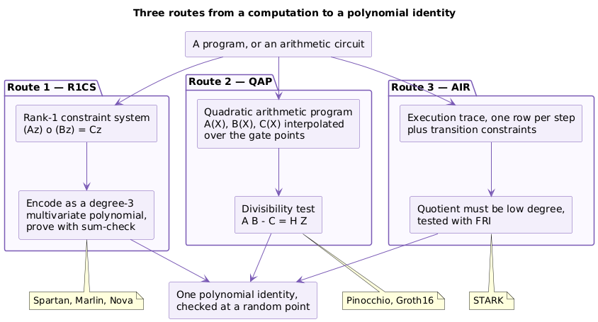
Every system discussed here does the same thing. It encodes a statement (“this program ran correctly on this input”) as a polynomial identity, then checks that identity at a single random point rather than everywhere. Two distinct polynomials of bounded degree agree in very few places, so agreeing at a random point is convincing evidence that they are the same polynomial. Everything else is engineering: how you build the polynomials, how you stop the prover from changing them mid-protocol, and what you assume is computationally hard.
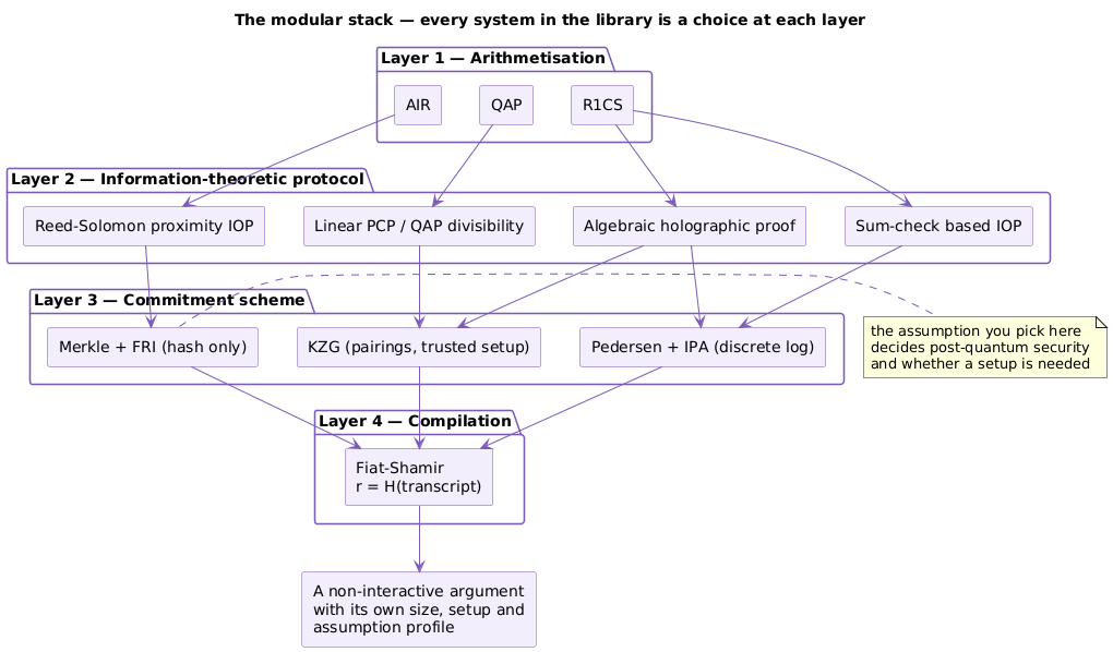
The papers differ in three choices, and almost nothing else:
- Arithmetisation. How the computation becomes polynomials (R1CS, QAP, or AIR).
- The information-theoretic protocol. What is proved about those polynomials, assuming the verifier can magically query them (sum-check, linear PCPs, proximity testing).
- The commitment scheme. What replaces that magic with real cryptography (pairings, discrete logs, or hashes).
Once you can name those three choices for a given paper, you can predict its proof size, its setup requirement, and whether a quantum computer breaks it.
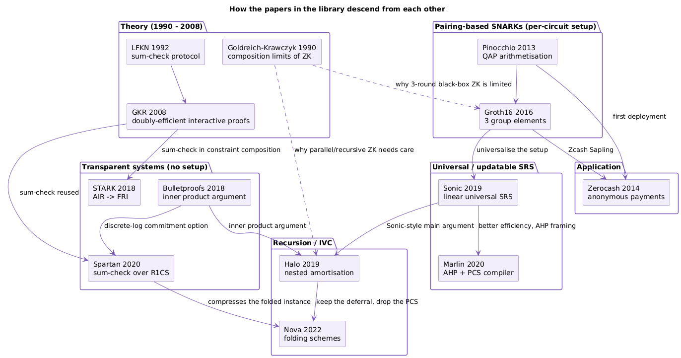
Part I — Fifteen Concepts
Group A: The engine underneath everything
1. Polynomial fingerprinting via Schwartz-Zippel
A non-zero polynomial of total degree \(d\) over a field \(\mathbb F\) has at most \(d\) roots, so a random point is very unlikely to be one. Comparing two objects therefore reduces to encoding each as a polynomial and comparing one evaluation.
This is the source of every soundness bound in the library. When a paper says “soundness error at most \(2^{-100}\)”, it almost always means “degree divided by field size, times the number of times we did this”. If you understand nothing else, understand that a proof system is a machine for converting a claim into a polynomial identity so that this lemma can be applied to it.
Where to read it: sumcheck.pdf in the course materials states and uses it directly.
2. Low-degree extension
A function on the boolean hypercube \(\{0,1\}^v\) is just a table of \(2^v\) values. Its low-degree extension (in the multilinear case, its multilinear extension) is the unique polynomial of degree at most 1 per variable that agrees with the table on the cube and is defined everywhere else too.
Uniqueness is the whole point. Because there is exactly one such polynomial, two parties who compute the extension of the same table get the same polynomial and agree at every point. Two parties with tables that differ in a single entry get polynomials that disagree almost everywhere. A table of a million entries becomes checkable with one field element.
Where to read it: gkrnotes.pdf and l12-gkr.pdf both build it from scratch.
3. The sum-check protocol
Given a \(v\)-variate polynomial \(g\) and a claimed value for \(\sum_{b \in \{0,1\}^v} g(b)\), the sum-check protocol reduces that claim to a single evaluation \(g(r_1, \ldots, r_v)\) in \(v\) rounds. Each round strips one variable: the prover sends a univariate polynomial, the verifier checks it against the previous round’s value, and only then picks the next random challenge.
The ordering matters more than the algebra. The prover commits before seeing the challenge, so it cannot back-fit. Sum-check is the single most reused component in the library: GKR is built on it, Spartan is built on it, and it appears inside the constraint composition step of STARKs.
Where to read it: sumcheck.pdf, then 2019-550.pdf (Spartan) to see it applied to a general NP statement.
Group B: Arithmetisation, or how a computation becomes algebra
4. R1CS as the common constraint language
A rank-1 constraint system describes a computation with three matrices \(A\), \(B\), \(C\) and a vector \(\mathbf z\) holding the constant 1, the public input, and the witness. Each row is one constraint saying that a linear combination of \(\mathbf z\) times another linear combination equals a third.
R1CS is NP-complete and generalises arithmetic circuit satisfiability, which is why it became the interchange format. Marlin, Spartan, and Nova all take R1CS as input. When a paper says “we support R1CS”, it means you can compile ordinary code to it with existing tooling and plug the paper’s machinery underneath.
Where to read it: 2019-550.pdf (Spartan) has a clean treatment.
5. QAPs and the divisibility criterion
A quadratic arithmetic program interpolates the columns of the constraint matrices into polynomials \(A(X)\), \(B(X)\), \(C(X)\) over a set of points, one point per gate. The witness satisfies the circuit exactly when the polynomial \(A(X)B(X) - C(X)\) vanishes at every gate point, which happens exactly when the vanishing polynomial \(Z(X)\) of those points divides it.
Satisfiability has become a divisibility question, and divisibility is checkable at one random point. This was the step that made general-purpose SNARKs practical.
Where to read it: 2013-279.pdf (Pinocchio) introduces it; 2016-260.pdf (Groth16) compresses the resulting proof to three group elements.
6. AIR, execution traces, and the quotient
An algebraic intermediate representation describes a computation as a table with one row per execution step and one column per register. A transition constraint is a polynomial relation that must hold between every pair of consecutive rows. Interpolate each column into a polynomial over a multiplicative subgroup, and “the constraint holds on every step” becomes “this expression vanishes on the whole subgroup”, which becomes “the quotient by the subgroup’s vanishing polynomial is a genuine low-degree polynomial”.
AIR is what makes STARK provers scale: the trace is uniform, so the constraints are described once regardless of how many steps the computation takes.
Where to read it: 2018-046.pdf, sections on AIR and APR.
Group C: The cryptographic layer
7. Bilinear pairings as one multiplication in the exponent
A pairing is a map \(e: \mathbb G_1 \times \mathbb G_2 \to \mathbb G_T\) satisfying \(e(g^a, h^b) = e(g,h)^{ab}\). Ordinary group operations let you add hidden values; a pairing lets you multiply two hidden values, exactly once, and compare the result.
That “exactly once” is the design constraint behind every pairing-based SNARK. QAP verification needs one multiplicative check between committed values, which is precisely one pairing product equation. It is also the reason these systems are not post-quantum: pairing groups rest on discrete logarithms.
Where to read it: 2016-260.pdf (Groth16), whose whole contribution is minimising this equation.
8. The setup spectrum: per-circuit, universal, updatable, transparent
Some systems need a structured reference string produced from secret randomness that must then be destroyed. The library covers four points on that spectrum:
- Per-circuit SRS (Pinocchio, Groth16). A fresh ceremony for every circuit. Change one line of the program and you run the ceremony again.
- Universal SRS (Sonic). One ceremony supports every circuit up to a size bound.
- Updatable SRS (Sonic, Marlin). Later participants can strengthen the string; it stays secure as long as one contributor was honest.
- Transparent (STARK, Bulletproofs, Spartan, Halo). No secret ever existed. Parameters come from hashing public data.
This axis is usually the deciding factor in deployment, and it is independent of proof size.
Where to read it: 2019-099.pdf (Sonic) for the universal and updatable construction.
9. Polynomial commitment schemes as a swappable module
A polynomial commitment binds the prover to a polynomial with one short value, then lets it prove evaluations at chosen points. Three families appear in the library, with different costs and different assumptions:
| Family | Commitment | Assumption | Setup | Proof size |
|---|---|---|---|---|
| KZG | one group element | pairings, q-type | trusted SRS | constant |
| Pedersen with an inner product argument | one group element | discrete log | none | logarithmic |
| Merkle tree with FRI | one hash | collision-resistant hash | none | polylogarithmic, large constants |
Swapping the family changes the system’s entire profile while leaving the protocol above it untouched. Spartan is explicit about this: the same sum-check core yields different verifier costs depending on the commitment you attach.
Where to read it: 2017-1066.pdf (Bulletproofs) for the discrete-log family, 2018-046.pdf for the hash-based one.
Group D: The modular view
10. Interactive oracle proofs and algebraic holographic proofs
An interactive oracle proof is an interactive proof in which the prover’s messages are oracles the verifier may query at a few positions rather than read in full. An algebraic holographic proof adds two restrictions: the oracles are polynomials, and the verifier never receives the circuit description either, only a holographic encoding of it.
The reason this abstraction matters is Marlin’s methodology: design a public-coin AHP, prove it sound information-theoretically, then compile it with any extractable polynomial commitment scheme to obtain a preprocessing zkSNARK. Design and cryptography are separated, and each can be improved independently. Most systems published since follow this recipe.
Where to read it: 2019-1047.pdf (Marlin), the section defining AHPs.
11. The inner product argument and logarithmic folding
To prove a statement about a length-\(d\) vector, split it in half, take a random linear combination of the halves, and recurse. After \(\log_2 d\) rounds, one scalar remains. Each round costs two group elements, so communication is logarithmic in the vector length.
The catch is at the end: the verifier must check that the folded generator matches a specific combination of the original generators, which is a multi-scalar multiplication linear in \(d\). That single check is why Bulletproofs verification is linear, and removing it from the recursive path is the entire contribution of Halo.
Where to read it: 2017-1066.pdf (Bulletproofs), then 2019-1021.pdf (Halo) for what to do about the linear step.
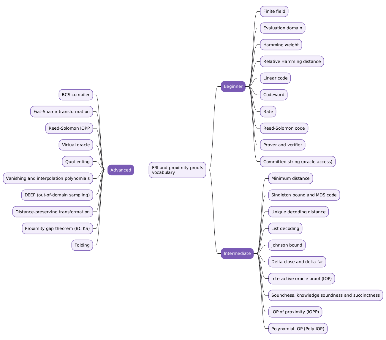
12. FRI and proximity to Reed-Solomon codes
FRI does not prove that a committed function is a low-degree polynomial. It proves that the function is close to one, in Hamming distance over the evaluation domain. That weaker guarantee is enough, because a function far from every low-degree polynomial cannot encode a satisfying assignment.
Mechanically it is a folding argument like the inner product argument, but over evaluations rather than group elements: split \(f\) into even and odd parts, combine them with a verifier challenge, halve the degree, repeat. Because it uses nothing but hashes and field arithmetic, it is the only construction here that is plausibly post-quantum.
Where to read it: 2018-046.pdf, the FRI section.
13. Fiat-Shamir and transcript binding
Replace each verifier challenge with a hash of everything sent so far. The protocol becomes non-interactive, and in the random oracle model it stays sound.
The subtlety is what “everything sent so far” means. If the hash omits the public parameters, the statement, or any prior message, a prover can grind: try candidate messages until the derived challenge is one it can answer for a false claim. Several deployed systems have been broken exactly here, and the fix is always the same, namely hash the full transcript. When reading any non-interactive system, find the transcript definition and check what it covers.
Where to read it: every paper applies it; 2019-1021.pdf (Halo) is notable because the transform has to be consistent inside and outside a circuit.
Group E: What the definitions actually promise
14. Soundness, knowledge soundness, and simulation
Three distinct guarantees are easy to confuse.
- Soundness says a false statement is rejected. It says nothing about a true statement whose prover has no idea why it is true.
- Knowledge soundness says more: whenever a prover convinces the verifier, an extractor with access to that prover can recover a witness. This is what “argument of knowledge” means, and it is the property that matters for a payment system, where “some valid coin exists” is useless and “this prover holds a valid coin” is the point.
- Zero knowledge is defined by a simulator that produces transcripts indistinguishable from real ones without any witness. If such a simulator exists, the transcript demonstrably carries no witness information.
The library also contains a paper about the limits of these definitions. Goldreich and Krawczyk show that the original zero-knowledge definition is not closed under sequential composition, that black-box simulation zero knowledge is not closed under parallel execution, and that only languages in BPP have three-round black-box simulation zero-knowledge interactive proofs. Those results explain why later constructions are careful about parallel repetition and round counts rather than treating them as free parameters.
Where to read it: Goldreich-Krawczyk.pdf.
15. Recursion: deferral versus folding
Recursive composition means a proof whose statement includes “the previous proof verified”. It gives incrementally verifiable computation: one constant-size proof for a computation of any length. It requires the verifier to be cheap enough to express as a circuit, and two papers here take different routes to that.
- Halo defers. It splits verification into a logarithmic part, which goes in the circuit, and the linear multi-scalar multiplication, which does not. The outstanding check is carried forward as a fixed-size deferred state, merged at every step, and paid once by the final verifier.
- Nova folds. Instead of proving anything per step, it combines two relaxed R1CS instances into one with a random linear combination. Folding is far cheaper than proving, so the per-step circuit is about 10,000 constraints. A single succinct proof is applied at the end to compress the result.
Both need a cycle of elliptic curves so that each step’s arithmetic is native to the curve it runs on.
Where to read it: 2019-1021.pdf (Halo) and 2021-370.pdf (Nova).
Concept-to-Paper Map
| # | Concept | Primary paper in the library |
|---|---|---|
| 1 | Schwartz-Zippel fingerprinting | sumcheck.pdf |
| 2 | Low-degree extension | gkrnotes.pdf, l12-gkr.pdf |
| 3 | Sum-check protocol | sumcheck.pdf, 2008-DelegatingComputation.pdf |
| 4 | R1CS | 2019-550.pdf (Spartan) |
| 5 | QAP and divisibility | 2013-279.pdf (Pinocchio) |
| 6 | AIR and execution traces | 2018-046.pdf (STARK) |
| 7 | Bilinear pairings | 2016-260.pdf (Groth16) |
| 8 | Setup spectrum | 2019-099.pdf (Sonic) |
| 9 | Polynomial commitments | 2017-1066.pdf (Bulletproofs) |
| 10 | IOPs and AHPs | 2019-1047.pdf (Marlin) |
| 11 | Inner product argument | 2017-1066.pdf (Bulletproofs) |
| 12 | FRI proximity testing | 2018-046.pdf (STARK) |
| 13 | Fiat-Shamir binding | all of them |
| 14 | Soundness, extraction, simulation | Goldreich-Krawczyk.pdf |
| 15 | Recursion: deferral and folding | 2019-1021.pdf, 2021-370.pdf |
Part II — Fifteen Formulas
These are the expressions that carry the arguments. Each is stated, then read out in words, because the notation is usually the only barrier.
F1. The Schwartz-Zippel bound
[\begin{aligned} \Pr_{r \,\leftarrow\, S^n}\bigl[P(r) = 0\bigr] \leq \frac{d}{\lvert S \rvert} \end{aligned}]
For a non-zero polynomial \(P\) in \(n\) variables of total degree \(d\), evaluated at a point drawn uniformly from \(S^n\) for a finite set \(S \subseteq \mathbb F\). Read it as: a non-zero polynomial is almost never zero at a random point. Concretely, with \(d = 2\) over a 128-bit field, the bound is about \(2^{-127}\).
F2. The multilinear extension
[\begin{aligned} \tilde f(x_1, \ldots, x_v) = \sum_{h \in {0,1}^v} f(h) \cdot \prod_{i=1}^{v} \bigl( h_i x_i + (1 - h_i)(1 - x_i) \bigr) \end{aligned}]
Each product term is a switch: it equals 1 at the corner \(h\) and 0 at every other corner. So the sum reproduces the table on the cube and interpolates smoothly elsewhere. This is the unique such polynomial with degree at most 1 per variable.
F3. The sum-check claim and its round consistency
[\begin{aligned} H = \sum_{b \in {0,1}^v} g(b), \qquad g_j(0) + g_j(1) = g_{j-1}(r_{j-1}), \qquad \varepsilon \leq \frac{v \cdot d}{\lvert \mathbb F \rvert} \end{aligned}]
The first is the claim. The second is the check the verifier performs in round \(j\), with \(g_0(r_0)\) defined to be \(H\): the two halves of the current round’s polynomial must reconstruct the previous round’s answer. The third is the resulting soundness error, with \(d\) the maximum degree in any single variable.
F4. Rank-1 constraint systems
[\begin{aligned} (A\mathbf z) \circ (B\mathbf z) = C\mathbf z, \qquad \mathbf z = (1,\ \mathbf x,\ \mathbf w) \end{aligned}]
Here \(\circ\) is the entrywise (Hadamard) product, \(\mathbf x\) is the public input and \(\mathbf w\) the witness. Row \(k\) says: one linear combination of \(\mathbf z\) multiplied by a second equals a third. Every arithmetic circuit can be written this way with one row per multiplication gate.
F5. The QAP divisibility criterion
[\begin{aligned} A(X) \cdot B(X) - C(X) = H(X) \cdot Z(X), \qquad Z(X) = \prod_{k=1}^{m} (X - \rho_k) \end{aligned}]
The polynomials \(A\), \(B\), \(C\) are witness-weighted combinations of fixed interpolation polynomials, one per wire. The points \(\rho_k\) are the gate labels. The identity holds for some polynomial \(H\) precisely when the constraint is satisfied at every gate. The verifier never checks every gate; it checks this identity at one secret point hidden in the SRS.
F6. The AIR transition constraint and its quotient
[\begin{aligned} C\bigl(T(x),\, T(\omega x)\bigr) = 0 \ \ \forall x \in H, \qquad Q(X) = \frac{C\bigl(T(X), T(\omega X)\bigr)}{Z_H(X)}, \qquad Z_H(X) = X^{\lvert H \rvert} - 1 \end{aligned}]
\(H\) is a multiplicative subgroup whose elements index the execution steps, and \(\omega\) is its generator, so \(\omega x\) is “the next step”. The constraint holding on every step is equivalent to \(Z_H\) dividing the constraint expression, which is equivalent to \(Q\) being a polynomial of the expected degree. Proving the computation reduces to proving \(Q\) has low degree.
F7. Pairing bilinearity
[\begin{aligned} e(g^a,\ h^b) = e(g, h)^{ab} \end{aligned}]
The exponents \(a\) and \(b\) are hidden inside group elements, yet their product appears in the target group. It works once: the output lives in \(\mathbb G_T\), which has no pairing of its own, so you cannot chain multiplications.
F8. The Groth16 verification equation
[\begin{aligned} e(A,\, B) = e(\alpha,\, \beta) \cdot e(L,\, \gamma) \cdot e(C,\, \delta) \end{aligned}]
\(A\), \(C\) and \(L\) are in \(\mathbb G_1\); \(B\), \(\alpha\), \(\beta\), \(\gamma\), \(\delta\) are the \(\mathbb G_2\) (and \(\mathbb G_1\)) setup elements. The proof is only \((A, B, C)\), three group elements. \(L\) is computed by the verifier from the public inputs. The whole QAP divisibility check has been folded into this one equation, evaluated with three pairings.
F9. KZG commitment and opening
[\begin{aligned} C = g^{p(\tau)}, \qquad q(X) = \frac{p(X) - v}{X - z}, \qquad \pi = g^{q(\tau)} \end{aligned}]
[\begin{aligned} e\bigl(C \cdot g^{-v},\ h\bigr) = e\bigl(\pi,\ h^{\tau} \cdot h^{-z}\bigr) \end{aligned}]
To prove \(p(z) = v\), the prover exhibits the quotient \(q\). That quotient is a polynomial exactly when \(X - z\) divides \(p(X) - v\), which happens exactly when \(p(z) = v\). The verifier checks divisibility in the exponent with one pairing equation. The secret \(\tau\) is never known to anyone; only its powers in the group are published.
F10. The Pedersen vector commitment
[\begin{aligned} \mathrm{Com}(\mathbf a;\ r) = \langle \mathbf a, \mathbf G \rangle + rH \end{aligned}]
The generators \(\mathbf G\) and \(H\) come from hashing public data, so nobody knows a discrete log relation among them. The commitment is perfectly hiding thanks to \(r\), computationally binding under the discrete log relation assumption, and additively homomorphic, which is what allows several openings to be batched into one.
F11. Inner product folding and the challenge vector
[\begin{aligned} \mathbf a’ = \mathbf a_{\mathrm{lo}} \cdot u + \mathbf a_{\mathrm{hi}} \cdot u^{-1}, \qquad \mathbf G’ = \mathbf G_{\mathrm{lo}} \cdot u^{-1} + \mathbf G_{\mathrm{hi}} \cdot u \end{aligned}]
[\begin{aligned} g(X, u_1, \ldots, u_k) = \prod_{i=1}^{k} \bigl( u_i + u_i^{-1} X^{2^{i-1}} \bigr) \end{aligned}]
The first line is one folding round: halve the vectors and recombine with the verifier’s challenge \(u\), using inverse exponents on the generators so the committed value is preserved. After \(k = \log_2 d\) rounds a single scalar remains. The second line is why the verifier survives: the length-\(d\) challenge vector implied by all the rounds has a product structure, so the scalar it induces costs \(O(\log d)\) to evaluate even though the corresponding group computation costs \(O(d)\). That asymmetry is the opening Halo exploits.
F12. The FRI folding step
[\begin{aligned} f(X) = f_e(X^2) + X \cdot f_o(X^2), \qquad f’(Y) = f_e(Y) + \beta \cdot f_o(Y) \end{aligned}]
Split the polynomial into its even-degree and odd-degree halves, then take a random combination chosen by the verifier. The degree halves at every step, so \(\log\) rounds reach a constant. The verifier spot-checks consistency between consecutive layers at randomly chosen positions, which is what turns this into a proximity test rather than an exact degree test.
F13. The Fiat-Shamir challenge
[\begin{aligned} r_j = H\bigl(\sigma,\ x,\ m_1,\ m_2,\ \ldots,\ m_j\bigr) \end{aligned}]
The \(j\)-th challenge is a hash of the public parameters \(\sigma\), the statement \(x\), and every prover message up to that point. Drop any argument from that list and you have created a grinding attack. This formula is short and is the most frequently implemented incorrectly.
F14. Knowledge soundness and the extractor
[\begin{aligned}
&\Pr\bigl[\langle P^\star, V\rangle(x) = 1\bigr] \geq \varepsilon
&\qquad \Longrightarrow \qquad \Pr\bigl[(x, w) \in R, \ \ w \leftarrow E^{P^\star}(x)\bigr] \geq \varepsilon - \kappa
\end{aligned}]
Here \(P^\star\) is any cheating prover, \(\langle P^\star, V\rangle(x)\) is the verifier’s output after interacting with it on statement \(x\), and \(R\) is the relation pairing statements with valid witnesses. If that prover convinces the verifier with probability at least \(\varepsilon\), then an extractor \(E\) with oracle access to it recovers a valid witness with probability at least \(\varepsilon\) minus the knowledge error \(\kappa\). This is the formal content of “the prover knows a witness”. Note what it does not say: nothing here claims the extractor is efficient enough to run in practice, and it is a thought experiment, never executed.
F15. Relaxed R1CS and the Nova folding step
[\begin{aligned} (A\mathbf z) \circ (B\mathbf z) = u \cdot (C\mathbf z) + \mathbf e \end{aligned}]
[\begin{aligned} \mathbf z \leftarrow \mathbf z_1 + r\,\mathbf z_2, \qquad u \leftarrow u_1 + r\,u_2, \qquad \mathbf e \leftarrow \mathbf e_1 + r\,\mathbf t + r^2\,\mathbf e_2 \end{aligned}]
The first line is R1CS relaxed with a scalar \(u\) and an error vector \(\mathbf e\). That relaxation is what makes the system closed under random linear combination: fold two satisfying instances and the result still satisfies the relaxed form, with \(\mathbf t\) absorbing the cross terms. Ordinary R1CS is the special case \(u = 1\) and \(\mathbf e = 0\). Folding costs two multi-scalar multiplications and no proof at all, which is why Nova’s per-step circuit is an order of magnitude smaller than Halo’s.
A Reading Order
The library is roughly chronological, but chronological is not the easiest path. Sum-check first, then one construction that uses it, then pick a branch.
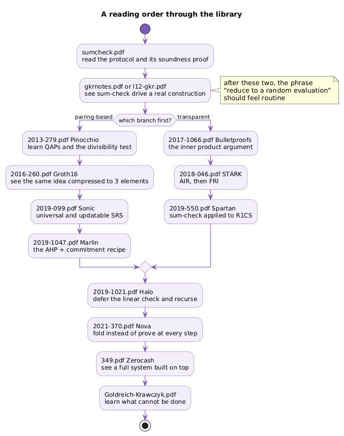
Two notes on using it. First, 2008-DelegatingComputation.pdf is the original GKR paper and is harder than the lecture notes covering the same protocol, so read gkrnotes.pdf or l12-gkr.pdf first and treat the paper as a reference. Second, 349.pdf (Zerocash) is worth reading early rather than last if you want motivation: it shows what the machinery is for, with coins as commitments, nullifiers preventing double spends, and Merkle membership proved in zero knowledge, all resting on a SNARK treated as a black box.
Conclusion
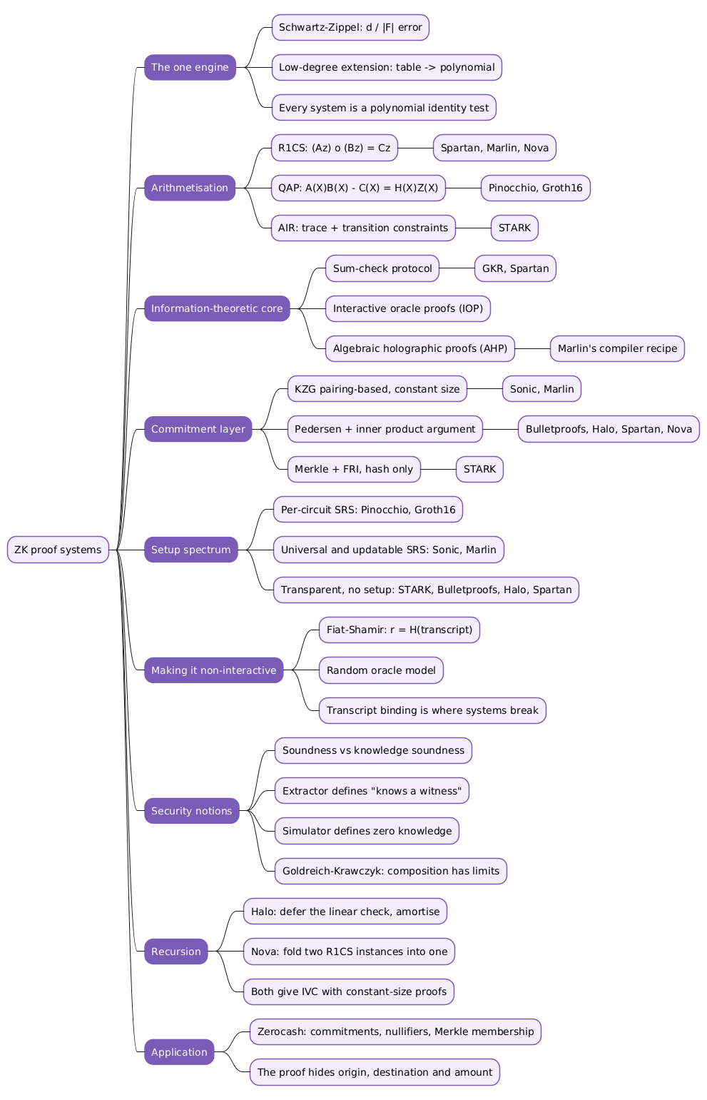
The fifteen concepts above are not fifteen independent things to memorise. Three of them (Schwartz-Zippel, low-degree extension, sum-check) are the mathematical engine. Three more (R1CS, QAP, AIR) are alternative front ends. Three are the cryptographic back ends (pairings, discrete-log commitments, hash-based commitments), and the setup spectrum follows from which back end you pick. The remaining six describe how the pieces are bolted together and what the resulting object is guaranteed to do.
The formulas map onto the same structure. F1 to F3 are the engine, F4 to F6 the front ends, F7 to F12 the back ends, and F13 to F15 the composition and recursion machinery.
A practical way to use this: for any paper in the library, answer four questions before reading past the introduction. Which arithmetisation does it use? What is the information-theoretic protocol underneath? Which commitment scheme instantiates it? What does the setup require? Four answers place the paper in the family tree, and the rest of the paper becomes the details of one particular route.
Annex
Key Terms
| Term | Definition |
|---|---|
| Arithmetisation | The step that turns a program or circuit into polynomials and polynomial constraints, so that correctness becomes an algebraic identity. |
| Low-degree extension | The unique polynomial of bounded degree per variable that agrees with a given table on the boolean hypercube and is defined over the whole field. |
| Sum-check protocol | A \(v\)-round reduction from a claimed sum of a polynomial over \(\{0,1\}^v\) to a single evaluation of that polynomial at a random point. |
| R1CS | A constraint system of the form \((A\mathbf z) \circ (B\mathbf z) = C\mathbf z\), used as the common input format by Marlin, Spartan and Nova. |
| QAP | A quadratic arithmetic program, which recasts circuit satisfiability as the divisibility of one polynomial by the vanishing polynomial of the gate points. |
| AIR | An algebraic intermediate representation: an execution trace plus polynomial constraints relating consecutive rows, used by STARKs. |
| Structured reference string (SRS) | Public parameters derived from secret randomness that must be discarded, classified as per-circuit, universal, or updatable. |
| Polynomial commitment scheme | A primitive binding a prover to a polynomial with one short value and allowing later proofs of its evaluations. |
| Interactive oracle proof (IOP) | An interactive proof in which prover messages are oracles the verifier queries at a few positions rather than reading in full. |
| Folding scheme | A primitive combining two instances of a relaxed constraint system into a single instance, cheaper than proving and used by Nova for recursion. |
Security Implementation Checklist
The properties below are the recurring places where a correct-on-paper proof system becomes an insecure deployed one. They apply across the constructions in the library, whichever layer choices a given system makes.
Field, parameters and arithmetisation
| Check | Security requirement | Failure mode if violated |
|---|---|---|
| ☐ | The field is large enough that (total degree) x (number of checks) divided by field size is negligible at the target security level. | Soundness degrades linearly with each reuse of Schwartz-Zippel; a small field makes a cheating prover’s guess feasible. |
| ☐ | Every constraint the computation relies on is actually present in the constraint system, including range and boolean constraints on witness values. | An under-constrained witness is the most common real-world proof-system bug: the proof verifies for values the program would never produce. |
| ☐ | Public inputs are bound into the statement the proof commits to, not passed alongside it. | An unbound public input lets a valid proof be replayed against different claimed inputs. |
Setup and reference string
| Check | Security requirement | Failure mode if violated |
|---|---|---|
| ☐ | For an SRS-based system, the ceremony transcript is public and verifiable, and at least one contributor is independent. | Whoever retains the trapdoor can forge proofs for false statements, undetectably. |
| ☐ | For a transparent system, generators are derived by hash-to-curve from a public seed, with no discrete log relation known among them. | A known relation among generators breaks the binding property of the commitment. |
| ☐ | The circuit a verification key was generated for is pinned and checked, and keys cannot be reset or replaced by an unprivileged party. | A swapped verification key turns the verifier into a rubber stamp for a circuit of the attacker’s choosing. |
Fiat-Shamir and challenge derivation
| Check | Security requirement | Failure mode if violated |
|---|---|---|
| ☐ | The transcript hashed for each challenge covers the public parameters, the statement, and every prior prover message. | Grinding: the prover searches for a message whose derived challenge lets a false claim pass. |
| ☐ | Domain separation distinguishes challenges at different protocol positions, and the hash output is at least twice the target security level in bits. | Cross-position challenge reuse, and collisions cheap enough to reintroduce adaptive attacks. |
| ☐ | Challenges required to be invertible are checked to be non-zero, with re-derivation rather than a default substitute on failure. | A predictable substituted challenge makes one folding or evaluation round non-binding. |
Commitments, openings and proof handling
| Check | Security requirement | Failure mode if violated |
|---|---|---|
| ☐ | Group elements received from a prover are validated: on-curve, in the prime-order subgroup, and non-identity where required. | Invalid-curve and small-subgroup inputs satisfy the verification equations without committing to anything. |
| ☐ | Declared degree bounds are enforced on every committed polynomial. | An over-degree polynomial escapes the argument’s structure, so the evaluation check no longer pins down the witness. |
| ☐ | For FRI-based systems, the number of query repetitions matches the claimed security level for the chosen code rate. | Too few queries let a function far from any low-degree polynomial pass the proximity test. |
| ☐ | Verification failure aborts; there is no path on which a partially checked proof is accepted. | A single skipped check is usually sufficient to accept arbitrary statements. |
Zero knowledge and recursion
| Check | Security requirement | Failure mode if violated |
|---|---|---|
| ☐ | Blinding randomness is fresh per proof and drawn from a CSPRNG. | Reused blinding lets two proofs be subtracted, recovering witness values. |
| ☐ | Zero knowledge is claimed only where a simulator argument exists; folding schemes such as Nova’s do not provide it natively. | Treating an intermediate folded instance as private leaks witness information. |
| ☐ | In a recursive chain, the base case is verified explicitly and the deferred or folded state is bound into each step’s public inputs. | An unverified base case or unbound state lets a chain attest to a state that was never computed. |
Frequently Asked Questions
Q: If everything reduces to checking a polynomial identity at a random point, why are there so many different systems?
Because the reduction is only half the problem. The verifier cannot actually evaluate the prover’s polynomial, since receiving it would cost as much as redoing the computation. So the polynomial has to be committed, and the commitment scheme is where the real trade-offs live. Pairing-based commitments give constant-size proofs but need a trusted setup and break under quantum attack. Discrete-log commitments need no setup but verify in linear time. Hash-based commitments assume almost nothing and survive quantum computers but produce proofs that are one or two orders of magnitude larger. Every system in the library is a different answer to that question, and the differences in arithmetisation follow from which commitment you intend to use.
Q: What is the actual difference between R1CS, QAP, and AIR? They all sound like ways of writing down a circuit.
They are, but they differ in what shape of computation they express naturally. R1CS is a flat list of constraints with no assumed structure, which makes it a good interchange format and a good match for sum-check, since the constraint system becomes a low-degree multivariate polynomial. A QAP is R1CS transformed into univariate polynomials interpolated over gate points, which converts satisfiability into a divisibility question that a pairing can check in one equation. AIR assumes the computation is a repeated state transition, so the constraints are described once and reused for every step, which is what lets a STARK prover scale to very long executions. Choosing AIR for a computation with no repetitive structure wastes its main advantage.
Q: Why does Bulletproofs verification take linear time when the proof is logarithmic in size?
The proof is short because the folding argument sends only two group elements per round, and there are \(\log_2 d\) rounds. But the last check requires the verifier to confirm that the folded generator equals a specific combination of all \(d\) original generators, and that is a multi-scalar multiplication over \(d\) elements. The corresponding scalar quantity is cheap, because the challenge vector has a product structure that F11 makes explicit, but the group computation has no such shortcut. Short proof, expensive verification, and the two are not in tension because they measure different things.
Q: How does Halo remove that linear check when it is inherent to the argument?
It does not remove it, it moves it. Halo splits verification into the logarithmic part and the linear multi-scalar multiplication, puts only the logarithmic part inside the recursive circuit, and carries the outstanding linear check forward as a fixed-size deferred state. Each step merges the new outstanding check into the accumulated one, so the state never grows. The final verifier, standing outside every circuit, performs the linear computation exactly once for the whole chain. The cost of verifying a million steps ends up close to the cost of verifying one.
Q: Which of these systems are broken by a quantum computer, and why is only one safe?
Pairing-based systems (Pinocchio, Groth16, Sonic, Marlin) and discrete-log systems (Bulletproofs, Halo, Spartan in its discrete-log instantiation, Nova) all rest on the hardness of discrete logarithms in some group, which Shor’s algorithm solves efficiently. STARKs rest only on collision resistance of a hash function, and the best known quantum attack on that is Grover’s algorithm, which merely halves the effective security level and is compensated by doubling the output size. So the dividing line is not the proof system’s design but the commitment scheme underneath it, which is another reason to read these papers in terms of their layers.
Q: Combining several of these ideas, why is knowledge soundness rather than plain soundness the property Zerocash needs?
Zerocash spends a coin by proving that a valid unspent coin exists in the Merkle tree and that its nullifier is being revealed. Plain soundness would only guarantee that such a coin exists somewhere in the tree, which is trivially true for any honest user’s coin and therefore proves nothing about the spender. What the system needs is that the party producing the proof actually holds the coin’s secret, and that is exactly what knowledge soundness formalises through the extractor of F14. This is also why the compilation step matters: Marlin’s recipe insists on an extractable polynomial commitment scheme, because a merely binding commitment would give an argument, not an argument of knowledge.
Q: The library has one paper that proves things cannot be done. Is it worth reading?
Yes, and reading it early saves time later. Goldreich and Krawczyk establish that the plain zero-knowledge definition does not survive sequential composition, that black-box simulation zero knowledge does not survive parallel execution, and that three-round black-box simulation zero-knowledge interactive proofs exist only for languages already in BPP. Those results are the reason later papers state their round complexity carefully, use auxiliary-input definitions of zero knowledge, and treat parallel repetition as something requiring proof rather than an obvious optimisation. Without that context, a lot of otherwise unmotivated care in the constructions looks arbitrary.
References
Theoretical foundations
- Goldreich, O., Krawczyk, H.: On the Composition of Zero-Knowledge Proof Systems. ICALP 1990. (
Goldreich-Krawczyk.pdf) - Lund, C., Fortnow, L., Karloff, H., Nisan, N.: Algebraic Methods for Interactive Proof Systems. JACM 1992. (Origin of the sum-check protocol.)
- Goldwasser, S., Kalai, Y. T., Rothblum, G. N.: Delegating Computation: Interactive Proofs for Muggles. STOC 2008. (
2008-DelegatingComputation.pdf) - Thaler, J.: Proofs, Arguments, and Zero-Knowledge. Lecture notes, 2022. (The modern successor to the COSC 544 course materials in the library.)
Pairing-based SNARKs
- Parno, B., Howell, J., Gentry, C., Raykova, M.: Pinocchio: Nearly Practical Verifiable Computation. IEEE S&P 2013. (
2013-279.pdf) - Groth, J.: On the Size of Pairing-Based Non-interactive Arguments. EUROCRYPT 2016. (
2016-260.pdf)
Universal and updatable setups
- Maller, M., Bowe, S., Kohlweiss, M., Meiklejohn, S.: Sonic: Zero-Knowledge SNARKs from Linear-Size Universal and Updatable Structured Reference Strings. CCS 2019. (
2019-099.pdf) - Chiesa, A., Hu, Y., Maller, M., Mishra, P., Vesely, N., Ward, N.: Marlin: Preprocessing zkSNARKs with Universal and Updatable SRS. EUROCRYPT 2020. (
2019-1047.pdf)
Transparent systems
- Bünz, B., Bootle, J., Boneh, D., Poelstra, A., Wuille, P., Maxwell, G.: Bulletproofs: Short Proofs for Confidential Transactions and More. IEEE S&P 2018. (
2017-1066.pdf) - Ben-Sasson, E., Bentov, I., Horesh, Y., Riabzev, M.: Scalable, transparent, and post-quantum secure computational integrity. IACR ePrint 2018. (
2018-046.pdf) - Setty, S.: Spartan: Efficient and general-purpose zkSNARKs without trusted setup. CRYPTO 2020. (
2019-550.pdf)
Recursion and incrementally verifiable computation
- Bowe, S., Grigg, J., Hopwood, D.: Recursive Proof Composition without a Trusted Setup. IACR ePrint 2019/1021. (
2019-1021.pdf) - Kothapalli, A., Setty, S., Tzialla, I.: Nova: Recursive Zero-Knowledge Arguments from Folding Schemes. CRYPTO 2022. (
2021-370.pdf)
Applications
- Ben-Sasson, E., Chiesa, A., Garman, C., Green, M., Miers, I., Tromer, E., Virza, M.: Zerocash: Decentralized Anonymous Payments from Bitcoin. IEEE S&P 2014. (
349.pdf)
Related articles
- KZG Polynomial Commitments — The Terms and Formulas, From Beginner to Advanced
- Understanding zk-SNARK: A Deep Dive into Zero-Knowledge Proofs
- Halo — Recursive Proof Composition without a Trusted Setup
- The GKR Protocol — Delegating Computation with Interactive Proofs
- Zero Knowledge Proofs with Bulletproof
- FRI and Proximity Proofs, Part 1 — Reed-Solomon Codes, IOPs of Proximity, Quotienting and Folding
You might also enjoy