KZG Polynomial Commitments — The Terms and Formulas, From Beginner to Advanced
Open a paper on Sonic, Marlin or PLONK and within a few pages you meet a commitment to a polynomial: one group element standing in for an object with thousands of coefficients, plus a second group element proving what that polynomial evaluates to at a chosen point. The construction is nearly always the same one, from a 2010 paper by Kate, Zaverucha and Goldberg, and it is normally cited rather than explained. It predates every zkSNARK that uses it, and it was written for verifiable secret sharing and credentials, not for proof systems.
The obstacle is the vocabulary. Words like witness, opening, evaluation binding, structured reference string and t-SDH carry precise meanings in that paper, and the SNARK literature reuses them without restating them. This article is a term list rather than a walkthrough: thirty terms split into three levels, each entry standalone, each with the formula that makes it concrete. Read it in order, or open it at whichever word stopped you. It is a companion to Zero-Knowledge Proof Systems — 15 Concepts and 15 Formulas to Read the Foundational Papers, which places the commitment layer inside the wider stack.
Afterwards you should be able to read the commitment section of any universal-SNARK paper without stopping, and say what a system gives up when it picks KZG over a hash-based or discrete-log alternative. The article defines the vocabulary; it does not walk through an implementation, and it does not build a proof system on top.
This article has been made with the help of Claude Code and several custom skills
Beginner — the objects and the assumptions
These terms name what the scheme handles and what it is built from. Nothing here depends on anything else in the article, and everything in the next level is assembled out of them.
Commitment scheme
A protocol that lets one party publish a short value fixing a choice, then reveal that choice later so anyone can check it was not changed in between. The published value is the commitment; revealing is opening.
The physical analogy is a sealed envelope: it is handed over first, opened afterwards. Two properties make it useful, and they pull in opposite directions. One stops the committer changing their mind, the other stops the receiver reading the envelope early.
Binding
The property that a committer cannot open one commitment to two different values. Once the commitment is published, the committed object is fixed.
Binding is what makes a commitment worth anything to the verifier. It comes in two strengths. Computationally binding means an attacker with bounded resources cannot find two openings, usually because doing so would solve a problem believed to be hard. Unconditionally binding means no two openings exist at all, regardless of computing power.
Hiding
The property that the commitment reveals nothing about the committed object until it is opened.
Hiding is the receiver-facing half of a commitment, and it mirrors binding in strength. Computationally hiding means an attacker with bounded resources learns nothing useful; unconditionally hiding means even an attacker with unlimited computing power learns nothing. A single scheme cannot be unconditional on both counts at once, so every construction picks which side to make unconditional.
Polynomial over a finite field
An expression \(\phi(x) = \phi_0 + \phi_1 x + \cdots + \phi_d x^d\) whose coefficients are drawn from \(\mathbb Z_p\), the integers modulo a prime \(p\), with all arithmetic done modulo \(p\).
Working over a finite field rather than the reals is what makes polynomials usable in cryptography: the coefficients are exact, they fit in a fixed number of bits, and they live in the same field as the exponents of a cryptographic group. A list of \(d+1\) messages can always be turned into a polynomial by interpolation, so committing to a polynomial also commits to a list.
Degree bound
The maximum degree \(t\) the scheme is set up to handle. The parameters are generated for a specific \(t\), and the committer may commit to any \(\phi(x)\) with \(\deg(\phi) \le t\).
The bound is not a formality. A polynomial of degree \(t\) is pinned down by any \(t+1\) of its values, so a committer who has opened that many points has no freedom left over the remaining ones, and a committer who has opened fewer still has some. The paper’s hiding definition is stated in exactly these terms, over the evaluations revealed so far. The public parameters have size \(O(t)\), which is the scheme’s main storage cost.
Polynomial commitment scheme
A commitment scheme whose committed object is a polynomial, and which additionally lets the committer prove individual evaluations \(\phi(i)\) without revealing the rest of the polynomial.
That second ability is what separates it from an ordinary commitment. Committing to the coefficients one by one works and costs \(t+1\) group elements; the point of the KZG construction is that the commitment stays a single element no matter how large \(t\) is. A Merkle tree over the evaluations is the closest familiar alternative, and its openings grow logarithmically rather than staying constant.
Generator and exponentiation in a group
A cyclic group \(\mathbb G\) of prime order \(p\) has a generator \(g\) such that every element is \(g^a\) for some \(a \in \mathbb Z_p\). Computing \(g^a\) from \(a\) is easy; recovering \(a\) from \(g^a\) is the discrete logarithm problem and is believed to be hard.
Everything below is built from that asymmetry. Exponents can be added and scaled behind the group operation, because \(g^a \cdot g^b = g^{a+b}\), so a value can be manipulated while staying hidden. What plain group arithmetic cannot do is multiply two hidden exponents together.
Bilinear pairing
A map that takes two group elements and returns one element of a third group, in a way that makes the hidden exponents multiply:
[\begin{aligned} e : \mathbb G \times \mathbb G \to \mathbb G_T, \qquad e(g^a,\ g^b) = e(g,g)^{ab} \end{aligned}]
Reading the letters: \(e\) is the pairing itself, \(\mathbb G\) is the source group and \(\mathbb G_T\) the target group, \(g\) is a generator of \(\mathbb G\), and \(a\) and \(b\) are the hidden exponents. Both arguments here come from the same \(\mathbb G\), which makes this the symmetric form; the 2010 paper uses it, and deployed curves use an asymmetric variant with two distinct source groups.
This is the operation ordinary groups lack, and it works once, because \(\mathbb G_T\) has no pairing of its own. KZG needs exactly one such multiplication, which is why one pairing equation verifies an opening.
Structured reference string (SRS)
Public parameters with algebraic structure, generated once from a secret value and published for everyone to use. For KZG the string is the tuple
[\begin{aligned} \mathrm{PK} = \bigl\langle g,\ g^{\alpha},\ g^{\alpha^2},\ \ldots,\ g^{\alpha^t} \bigr\rangle \end{aligned}]
for a secret \(\alpha\) drawn at random from the non-zero elements of \(\mathbb Z_p\). Anyone holding \(\alpha\) can forge openings, so \(\alpha\) must be destroyed after generation and is never needed again by the scheme. The contrast is with a transparent setup, where the parameters come from hashing public data and no secret ever exists.
Evaluation proof (witness)
The short value a committer sends alongside a claimed evaluation \(\phi(i)\) so that a verifier can confirm the claim is consistent with the published commitment. The 2010 paper calls it the witness and writes it \(w_i\); the SNARK literature usually calls it the opening proof or the opening.
In KZG the witness is a single group element, and it stays a single element whether the polynomial has ten coefficients or a million. Its size is independent of both the degree and the index being opened, which is the property the whole construction exists to deliver.
Intermediate — how the construction works
This level assumes the beginner terms and covers the machinery: how the commitment is formed, why an opening is checkable at all, and what the two published variants trade against each other.
Commitment in the exponent
The KZG commitment to \(\phi(x)\) is the polynomial evaluated at the secret \(\alpha\), carried in the exponent of the generator:
[\begin{aligned} C = g^{\phi(\alpha)} = \prod_{j=0}^{\deg(\phi)} \bigl(g^{\alpha^j}\bigr)^{\phi_j} \end{aligned}]
The committer never learns \(\alpha\). It only combines the published powers \(g^{\alpha^j}\) using its own coefficients \(\phi_j\) as exponents, which is why the right-hand form matters: it is the recipe an honest committer runs. The result is one group element, and the degree is bounded implicitly because the string stops at \(g^{\alpha^t}\), an argument that needs its own assumption to be made precise.
Polynomial remainder theorem
For any polynomial \(\phi(x)\) and any index \(i\), the linear factor \(x - i\) divides \(\phi(x) - \phi(i)\) exactly, with no remainder:
[\begin{aligned} \phi(x) - \phi(i) = (x - i)\,\psi_i(x) \end{aligned}]
The rest of the construction is this fact carried into a group. It turns the statement “\(\phi\) evaluates to \(\phi(i)\) at \(i\)” into the statement “this division comes out even”, and divisibility is something a pairing can check without either party revealing \(\phi\). Every KZG opening is a demonstration of exact division.
Quotient polynomial
The polynomial left over after dividing out the linear factor, written \(\psi_i(x)\) and computed by the committer as
[\begin{aligned} \psi_i(x) = \frac{\phi(x) - \phi(i)}{x - i}, \qquad w_i = g^{\psi_i(\alpha)} \end{aligned}]
The witness is this quotient committed the same way the polynomial itself was, and its degree is \(\deg(\phi) - 1\), so an honest committer can always build it from the same public parameters. The intuition for soundness is that a wrong claimed value leaves a non-zero remainder, so the quotient is a rational function rather than a polynomial and cannot be committed from the reference string. The proof itself is a reduction: a committer who produces a passing witness for a wrong value can be turned into a solver for t-SDH.
VerifyEval pairing equation
The single check a verifier runs to accept a claimed evaluation:
[\begin{aligned} e(C,\ g) \;\overset{?}{=}\; e\bigl(w_i,\ g^{\alpha}/g^{i}\bigr) \cdot e(g,g)^{\phi(i)} \end{aligned}]
Reading it in the exponent makes it obvious. The right-hand side is \(e(g,g)^{\psi_i(\alpha)(\alpha - i) + \phi(i)}\), and the remainder theorem says that exponent is exactly \(\phi(\alpha)\), which is the left-hand side. The verifier needs only \(g^{\alpha}\) from the reference string, so verification cost does not grow with \(t\).
PolyCommitDL
The paper’s first construction, written with a DL subscript because its hiding property rests on the discrete logarithm assumption. It is the scheme described by the three entries above: commitment \(C = g^{\phi(\alpha)}\), witness \(w_i = g^{\psi_i(\alpha)}\), one pairing check.
Its binding property rests on the t-SDH assumption, and its hiding is computational. This is the variant every zkSNARK means when it says “KZG”, because a proof system normally supplies its own blinding rather than relying on the commitment for zero knowledge.
PolyCommitPed
The paper’s second construction, named after Pedersen commitments, which adds a random polynomial \(\hat\phi(x)\) against a second generator \(h\):
[\begin{aligned} C = g^{\phi(\alpha)} h^{\hat\phi(\alpha)} \end{aligned}]
The trade is the standard one. Hiding becomes unconditional, so an attacker with unlimited computing power still learns nothing about unopened evaluations, while binding stays computational under t-SDH. The cost is a reference string of \(2t+2\) elements instead of \(t+1\), and a witness that carries a second exponentiation.
Polynomial binding
The security requirement that no efficient adversary can produce one commitment \(C\) together with two distinct polynomials \(\phi(x) \ne \phi'(x)\) that both verify against it.
This is binding in its ordinary sense, applied to the whole committed object. It is the weaker of the paper’s two requirements, because it says nothing about a committer who never opens the full polynomial and instead lies about a single evaluation. Real protocols rarely open the whole polynomial, which is why the second notion exists.
Evaluation binding
The stronger requirement that no efficient adversary can produce two accepting openings of the same commitment at the same index with different values, that is two triples \(\langle i, v, w\rangle\) and \(\langle i, v', w'\rangle\) that both verify with \(v \ne v'\).
This is the property protocols rely on, since a verifier sees evaluations and never the polynomial. Polynomial binding stops the committer swapping the object; evaluation binding stops it lying about one point of an object it never fully discloses. A scheme can satisfy the first and be useless without the second.
Additive homomorphism
The property that commitments combine under the group operation the way their polynomials combine under addition. For \(\phi = \phi_1 + \phi_2\):
[\begin{aligned} C_{\phi} = C_{\phi_1} \cdot C_{\phi_2}, \qquad w_{\phi,i} = w_{\phi_1,i} \cdot w_{\phi_2,i} \end{aligned}]
An opening of a sum can therefore be assembled from openings of the parts. This is what lets later protocols take a random linear combination of many committed polynomials and open the combination once instead of opening each one, and it is also how PolyCommitPed is built out of two commitments under different generators.
Batch opening
Opening a whole set of indices \(B\) with one witness rather than one per index. The committer divides by the vanishing polynomial of the set and commits to the quotient:
[\begin{aligned} \psi_B(x) = \frac{\phi(x) - r(x)}{\prod_{i \in B}(x - i)}, \qquad w_B = g^{\psi_B(\alpha)} \end{aligned}]
Here \(r(x)\) is the remainder of that division, and it interpolates the opened values, so \(r(i) = \phi(i)\) for every \(i \in B\). Revealing \(k\) of \(t\) committed values therefore costs \(O(k)\) to transmit \(r\) plus one group element, instead of \(k\) separate witnesses. Its binding rests on t-BSDH rather than t-SDH.
Advanced — assumptions, limits and downstream use
This level assumes the mechanics above. It covers the hardness assumptions the security proofs name, the properties the 2010 paper does not provide, and what changes when the scheme is dropped into a proof system.
t-Strong Diffie-Hellman assumption (t-SDH)
The assumption that, given the reference string \(\langle g, g^{\alpha}, \ldots, g^{\alpha^t}\rangle\), no efficient adversary can output a pair
[\begin{aligned} \bigl(c,\ g^{1/(\alpha + c)}\bigr), \qquad c \in \mathbb Z_p \setminus {-\alpha} \end{aligned}]
Introduced by Boneh and Boyen, it is the assumption underneath binding for both KZG constructions. It is a q-type assumption: its statement is parameterised by \(t\), and the larger \(t\) is the more the adversary is given, so a bigger degree bound is a stronger assumption rather than the same one. Cheon’s attack turns that into a measurable loss, recovering \(\alpha\) faster as the published powers extend, which is why deployed parameters are chosen with the intended \(t\) in mind.
t-Bilinear Strong Diffie-Hellman assumption (t-BSDH)
The same problem moved into the target group: the adversary must produce \(\bigl(c,\ e(g,g)^{1/(\alpha+c)}\bigr)\) from the same reference string.
Batch opening needs this variant rather than plain t-SDH, because its verification equation compares elements of \(\mathbb G_T\) that the single-point equation never forms. It is a distinct assumption, so a protocol that batches openings rests on slightly different ground from one that opens points individually.
t-polynomial Diffie-Hellman assumption (t-polyDH)
The assumption that, from a reference string ending at \(g^{\alpha^t}\), no efficient adversary can output a pair
[\begin{aligned} \bigl\langle \phi(x),\ g^{\phi(\alpha)} \bigr\rangle, \qquad t \lt \deg(\phi) \lt 2^{\kappa} \end{aligned}]
for security parameter \(\kappa\). The upper bound is not decoration: for degrees near the field size the value is computable by other means, since \(\phi(x) = x^{p-1}\) gives \(g^{\phi(\alpha)} = g\) for every non-zero \(\alpha\). This is the assumption that makes the degree bound meaningful, because without it the claim that a truncated reference string confines the committer to degree \(t\) is an intuition rather than a hypothesis. The paper introduces it as a generalisation of the t-DHI assumption.
Trapdoor and the powers-of-tau ceremony
The secret \(\alpha\) is a trapdoor: anyone who knows it can compute \(g^{\phi(\alpha)}\) for any polynomial and open any commitment to any value, undetectably. The scheme’s binding is therefore conditional on that value being gone.
Since a single trusted dealer is a weak assumption, deployments generate the string through a multi-party ceremony in which each contributor mixes in fresh randomness and destroys it. The string is sound if at least one participant was honest, and the discarded randomness is what the ecosystem calls toxic waste. Ethereum’s KZG ceremony for proto-danksharding collected over 140,000 contributions on this argument.
Degree bound enforcement
Verification checks that an evaluation is consistent with the commitment; it does not check that the committed polynomial has any particular degree. The reference string caps the degree at \(t\) under t-polyDH, but a protocol that needs a tighter bound \(d \lt t\) gets no help from the pairing equation.
The standard fix, introduced by later work rather than the 2010 paper, is a shifted commitment: commit to \(x^{t-d}\,\phi(x)\) as well and check the two are consistent. Only a polynomial of degree at most \(d\) shifts into the available range. Sonic and Marlin build an explicit degree bound into their commitment scheme this way; systems that instead lean on the reference string’s length are sound only when the bound they need is the one the string already gives.
Algebraic Group Model (AGM)
An idealised model in which every adversary that outputs a group element must also output the coefficients expressing it as a combination of the elements it was given.
It sits between the standard model and the generic group model: weaker than assuming the adversary cannot look inside group elements, stronger than assuming nothing. KZG’s use in SNARKs is normally proved here, because the security notion those proofs need is not implied by binding alone and has no known proof from a falsifiable assumption.
Extractability
The property that any adversary producing a valid commitment and opening must “know” an underlying polynomial, in the formal sense that an efficient extractor can recover it from the adversary.
Binding says two openings cannot both verify. Extractability says something stronger: that a polynomial exists and is recoverable. A proof system needs this because knowledge soundness is a statement about the prover possessing a witness, and a merely binding commitment leaves room for a prover that convinces without knowing anything. This is the property proved in the AGM, and the reason a paper will specify “extractable polynomial commitment” rather than just “polynomial commitment”.
Symmetric and asymmetric pairings
The paper’s pairing is type 1, or symmetric: one source group used for both arguments. It says it chose that only to simplify presentation, and that the constructions carry over to the other types. Deployed systems use type 3, or asymmetric, with two distinct source groups and no efficiently computable map between them:
[\begin{aligned} e : \mathbb G_1 \times \mathbb G_2 \to \mathbb G_T, \qquad e(g_1^a,\ g_2^b) = e(g_1, g_2)^{ab} \end{aligned}]
Type 2 sits between the two, with a homomorphism in one direction only. Type 1 is avoided because its low embedding degree forces a large base field to reach a useful security level, and because such parameters have repeatedly been weakened by advances in discrete-logarithm algorithms. Reading the paper against a BLS12-381 implementation therefore means assigning each element to one of the two groups: library code puts \(g^{\alpha}\) in \(\mathbb G_2\) and the commitment in \(\mathbb G_1\).
Compiling a polynomial IOP into a SNARK
The pattern that made KZG central to the field: describe a proof system in an idealised model where the verifier may query polynomials at arbitrary points for free, then replace each idealised polynomial with a commitment and each query with an opening.
The idealised protocol supplies soundness, the commitment supplies the cryptography, and the two are designed independently. Sonic, Marlin and PLONK are all this compiler applied to different idealised protocols, which is why they share a setup model and differ mostly in prover cost. Swapping the commitment for a hash-based one turns the same protocol transparent.
Post-quantum exposure
Every security property above rests on discrete logarithms in a pairing group, which Shor’s algorithm solves. A sufficiently large quantum computer recovers \(\alpha\) from the reference string and destroys binding for every commitment ever made under it, retroactively.
That is why a system aiming at post-quantum plausibility does not use KZG. FRI commits through Merkle trees over Reed-Solomon codewords and needs only a collision-resistant hash, at the price of proofs measured in kilobytes; the Bulletproofs inner product argument needs only discrete logarithms and no setup, at the price of logarithmic proofs and linear verification. The choice among the three is a choice among constant proofs, no trusted setup, and quantum resistance, and no deployed scheme offers all three.
Conclusion
The vocabulary has one load-bearing idea and a lot of consequences. The polynomial remainder theorem is what makes an evaluation checkable at all, and everything in the intermediate level is that fact expressed in a group: the quotient becomes the witness, the division becomes a pairing equation, and the degree bound becomes the length of the reference string. A reader who can rederive the verification equation from the remainder theorem has the construction.
The intermediate level is the real threshold, and the entry that most often separates a working understanding from a partial one is evaluation binding, because it is the property protocols use and the one polynomial binding does not imply. The advanced level is where the caveats live: the degree bound the pairing check does not enforce, the extractability that binding does not give, and the trapdoor whose destruction the whole scheme assumes. Next, read the KZG section of Marlin or PLONK, where these terms appear in their working form, and compare it against the FRI construction to see which of the properties above are consequences of pairings rather than of commitment schemes in general.
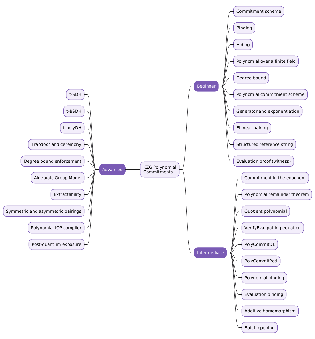
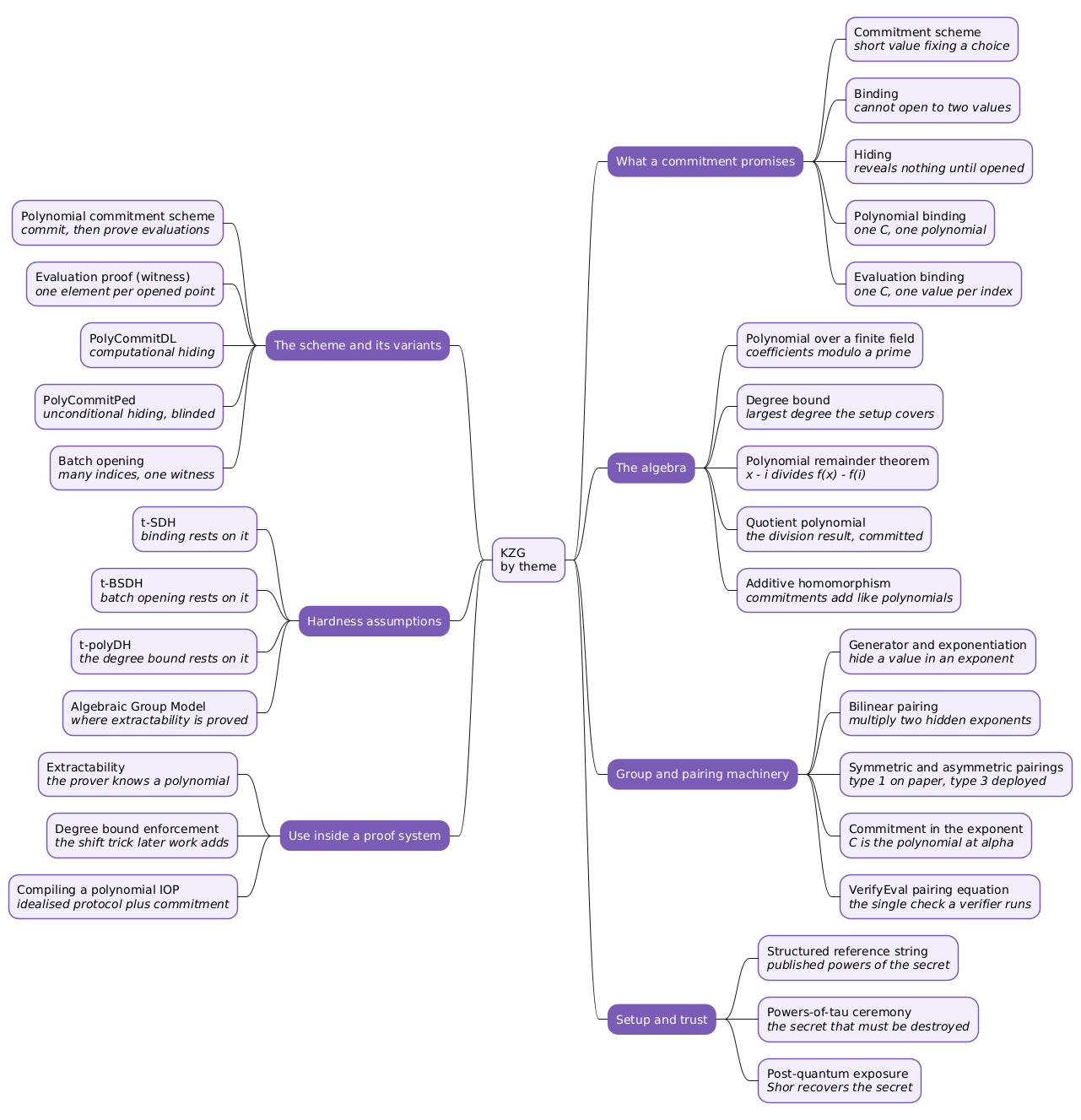
Sorted by reading order the vocabulary is three levels deep. Sorted by subject it is seven clusters, and the second cut shows which entries are one idea split across levels: binding is a beginner term whose two precise forms are intermediate, while the assumptions and the proof-system machinery sit entirely in the advanced level.
Frequently Asked Questions
Q: What is the difference between binding and hiding?
Binding protects the verifier: once a commitment is published, the committer cannot open it to a different value. Hiding protects the committer: the published commitment leaks nothing about what was committed.
They are separate requirements, and each comes in a computational and an unconditional flavour. No scheme is unconditional on both at once, which is exactly the axis separating the paper’s two constructions: PolyCommitDL has computational hiding, PolyCommitPed has unconditional hiding, and both have computational binding.
Q: Why does an opening need a quotient polynomial rather than just the claimed value?
Because the claimed value on its own is unverifiable. The verifier holds one group element and cannot evaluate the committed polynomial itself.
The quotient turns the claim into an algebraic fact the verifier can test. By the polynomial remainder theorem, \(\psi_i(x) = (\phi(x) - \phi(i))/(x - i)\) is a genuine polynomial precisely when \(\phi(i)\) is the correct value; if the value is wrong, the division leaves a remainder and no such polynomial exists. Turning that into a security claim takes the t-SDH reduction, which converts a passing witness for a wrong value into a solution to the assumed-hard problem. The VerifyEval pairing equation is the check that the division came out even.
Q: What is the difference between polynomial binding and evaluation binding?
Polynomial binding says one commitment cannot verify against two different polynomials. It concerns the whole committed object.
Evaluation binding says one commitment cannot produce two accepting openings at the same index with different values. It concerns a single point of an object that is never fully revealed.
The second is what protocols rely on, because a verifier in a proof system sees evaluations and never the polynomial. A scheme could satisfy polynomial binding and still let a committer lie about one evaluation, which would make it useless in practice.
Q: What happens if the powers-of-tau ceremony is compromised?
Binding disappears entirely, and silently. Someone holding \(\alpha\) can compute a commitment in the exponent for any polynomial, and can produce a passing witness for any value at any index, because they can evaluate every quantity the pairing equation compares. Nothing distinguishes such a forgery from an honest opening.
Two things limit the damage. The ceremony is secure if at least one participant destroyed their contribution, so an attacker must compromise every participant rather than any one of them. And hiding is unaffected in PolyCommitPed, whose hiding is unconditional and therefore independent of the trapdoor.
Q: What does batch opening save?
It replaces \(k\) witnesses with one. Opening \(k\) indices separately costs \(k\) group elements and \(k\) verification equations; batching costs one group element plus the interpolating remainder \(r(x)\), checked in a single equation.
Note which direction it batches: one polynomial opened at many indices. The mirror case, many polynomials opened at one index, is handled instead by additive homomorphism, by opening a random linear combination of the commitments. Proof systems use both. The cost of the batch here is a different hardness assumption: batch opening rests on t-BSDH rather than t-SDH, because its verification equation compares elements the single-point equation never forms.
Q: When would you choose KZG over a hash-based polynomial commitment scheme such as FRI?
Choose KZG when proof size and verification cost dominate, and a setup ceremony is acceptable. It gives a constant-size commitment, a constant-size opening, and a verifier whose work does not grow with the degree bound, which is why on-chain verification generally uses it.
Choose a hash-based commitment when the setup is unacceptable or post-quantum exposure matters. It needs no trapdoor and no pairing-friendly curve, at the price of proofs measured in kilobytes rather than bytes. The compiler that turns a polynomial IOP into a SNARK is indifferent to which one is plugged in, so this is a deployment decision rather than a protocol one.
Notation — the Greek letters used
The formulas use a small, fixed set of Greek symbols. Two rows below name the same object, because the paper and the deployments spell it differently.
| Symbol | Name | What it stands for here |
|---|---|---|
| \(\alpha\) | alpha | The setup secret. The reference string is its successive powers \(g^{\alpha^j}\), and it is the trapdoor that must be destroyed after generation. |
| \(\tau\) | tau | The same secret as \(\alpha\), under the name most deployments use. This article writes \(\alpha\) with the paper, but the ceremony that produces the string is universally called powers-of-tau. |
| \(\phi\) | phi | The committed polynomial. \(\phi(x)\) is the polynomial, \(\phi(i)\) its evaluation at index \(i\), and \(\phi_j\) its coefficient of \(x^j\). |
| \(\hat\phi\) | phi-hat | The random blinding polynomial that PolyCommitPed adds against the second generator \(h\) to make hiding unconditional. |
| \(\psi\) | psi | The quotient polynomial that becomes the witness: \(\psi_i\) when opening one index, \(\psi_B\) when batching a set \(B\). |
| \(\kappa\) | kappa | The security parameter, which bounds how large a degree the t-polyDH assumption covers. |
| \(\prod\) | capital pi | An operator rather than a variable: the product over a range. It builds the commitment from the reference string, and forms the vanishing polynomial \(\prod_{i \in B}(x-i)\) in batch opening. |
The Latin letters follow the paper as well: \(g\) and \(h\) are generators, \(C\) a commitment, \(w\) a witness, \(t\) the degree bound, \(i\) an index, and \(e\) the pairing.
References
Primary source
- Kate, A., Zaverucha, G. M., Goldberg, I.: Constant-Size Commitments to Polynomials and Their Applications. ASIACRYPT 2010, LNCS 6477, pp. 177-194. The security proofs are in the extended version, referenced in the paper as [24].
Underlying assumptions
- Boneh, D., Boyen, X.: Short Signatures Without Random Oracles. EUROCRYPT 2004. (Origin of the t-SDH assumption.)
- Cheon, J. H.: Security Analysis of the Strong Diffie-Hellman Problem. EUROCRYPT 2006.
- Fuchsbauer, G., Kiltz, E., Loss, J.: The Algebraic Group Model and its Applications. CRYPTO 2018.
Proof systems built on it
- Maller, M., Bowe, S., Kohlweiss, M., Meiklejohn, S.: Sonic: Zero-Knowledge SNARKs from Linear-Size Universal and Updatable Structured Reference Strings. CCS 2019.
- Chiesa, A., Hu, Y., Maller, M., Mishra, P., Vesely, N., Ward, N.: Marlin: Preprocessing zkSNARKs with Universal and Updatable SRS. EUROCRYPT 2020.
- Gabizon, A., Williamson, Z. J., Ciobotaru, O.: PlonK: Permutations over Lagrange-bases for Oecumenical Noninteractive arguments of Knowledge. IACR ePrint 2019/953.
- Groth, J.: On the Size of Pairing-Based Non-interactive Arguments. EUROCRYPT 2016.
The alternatives
- Ben-Sasson, E., Bentov, I., Horesh, Y., Riabzev, M.: Fast Reed-Solomon Interactive Oracle Proofs of Proximity. ICALP 2018. (FRI.)
- Bünz, B., Bootle, J., Boneh, D., Poelstra, A., Wuille, P., Maxwell, G.: Bulletproofs: Short Proofs for Confidential Transactions and More. IEEE S&P 2018.
Related articles
- FRI and Proximity Proofs — The Vocabulary, From Beginner to Advanced
- Zero-Knowledge Proof Systems — 15 Concepts and 15 Formulas to Read the Foundational Papers
- Understanding zk-SNARK: A Deep Dive into Zero-Knowledge Proofs
- Halo — Recursive Proof Composition without a Trusted Setup
- Zero Knowledge Proofs with Bulletproof
- FRI and Proximity Proofs, Part 1 — Reed-Solomon Codes, IOPs of Proximity, Quotienting and Folding
You might also enjoy