FRI and Proximity Proofs — The Vocabulary, From Beginner to Advanced

By Ryan S. · 2026, Sep 11

FRI is the proximity test at the bottom of every STARK and of most hash-based SNARKs. A prover commits to a long table of field elements, and a verifier who reads a few dozen of its entries becomes convinced that the whole table is close to the evaluations of a low-degree polynomial. Open any paper in this line of work, from the original FRI to DEEP-FRI, the proximity gaps theorem or STIR, and the same words return on every page: rate, list decoding, Johnson bound, IOP of proximity, quotient, out-of-domain sample, folding.

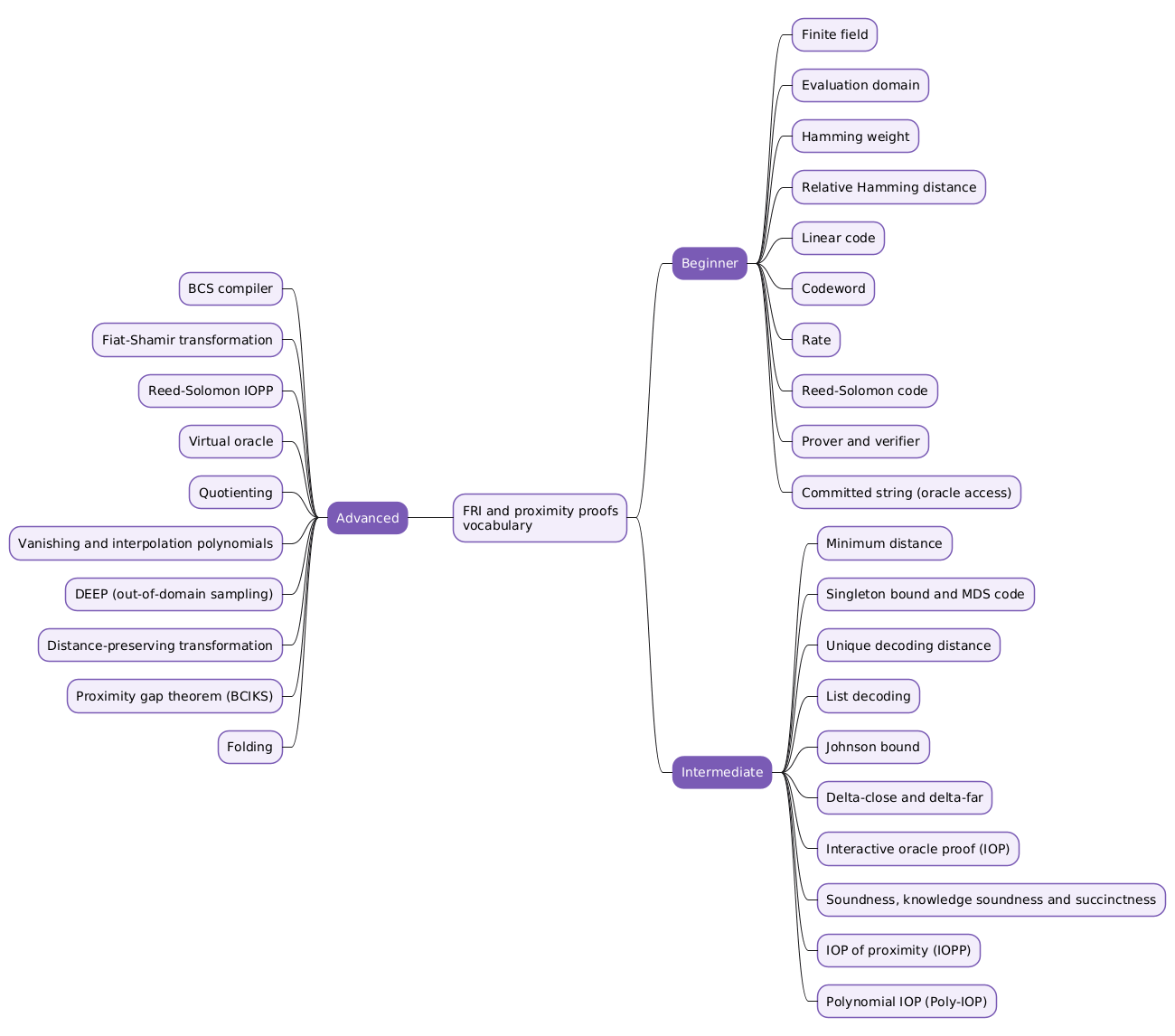
Those words are the obstacle. Each carries a precise meaning borrowed from coding theory or from the theory of interactive proofs, and the papers reuse them without restating them. This article is a term list rather than a walkthrough: thirty terms split into three levels, each entry standalone, each with the formula or the fact that makes it concrete. Read it in order, or open it at whichever word stopped you.

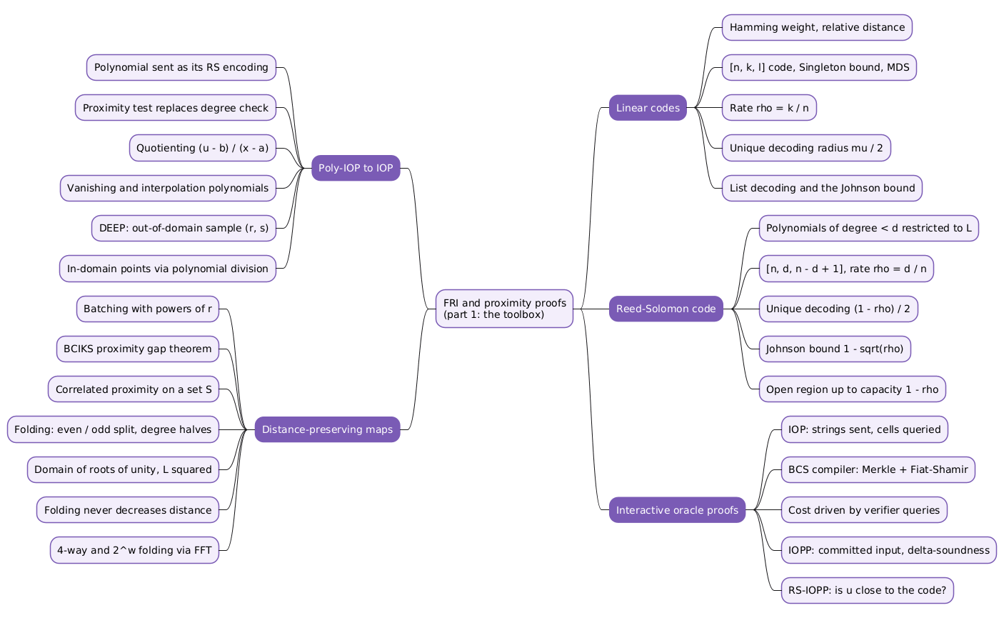
The terms are those used in the first half of a two-part ZK Whiteboard Sessions lecture by Dan Boneh on FRI, and in its companion article on this site, FRI and Proximity Proofs, Part 1 — Reed-Solomon Codes, IOPs of Proximity, Quotienting and Folding, which walks through the constructions. This one defines the vocabulary; it does not build the protocol.

This article has been made with the help of Claude Code and several custom skills

Beginner — the objects

These terms name the things the protocol handles: the field, the domain, the words, the code and the two parties. Nothing here depends on anything else in the article, and every later term is assembled from these.

Finite field

A set of $p$ elements, for $p$ a prime, written $\mathbb F = \{0, 1, \dots, p-1\}$, in which addition and multiplication are performed modulo $p$, so that every non-zero element has an inverse.

Every value in FRI, from the entries of a committed table to the verifier’s random challenges, is a field element. The field’s size matters twice over: it must be large enough for random challenges to be unpredictable, and, for FRI specifically, $p - 1$ must be divisible by the size of the evaluation domain so that a suitable group of roots of unity exists.

Evaluation domain

A fixed subset $L \subseteq \mathbb F$ of size $n$ at whose points polynomials are evaluated. Its elements are given a fixed order, so a function $u : L \to \mathbb F$ and a vector in $\mathbb F^n$ are two views of the same object.

In FRI the domain is not arbitrary: $n$ is a power of two and $L$ is the set of $n$-th roots of unity, which makes $x \in L$ imply $-x \in L$. That symmetry is what later allows folding. Points outside $L$, written $\mathbb F \setminus L$, are where evaluation queries and out-of-domain samples are taken.

Hamming weight

The number of non-zero coordinates of a vector $u \in \mathbb F^n$, written $\lVert u \rVert_0$ and sometimes called the zero norm.

A compact formula is $\lVert u \rVert_0 = \sum_i u_i^{\,0}$ with the convention $0^0 = 0$, so each non-zero coordinate contributes one and each zero coordinate nothing. It behaves like a norm, including the triangle inequality, which is the single property most arguments about codes rely on.

Relative Hamming distance

The fraction of coordinates on which two vectors of the same length differ:

[\begin{aligned} \Delta(u, v) = \frac{\lVert u - v \rVert_0}{n} \in [0, 1]. \end{aligned}]

Normalising by $n$ lets statements about closeness be made independently of the length of the vectors. Two words of length five that differ in three positions are at relative distance $3/5$. All the radii that follow, the unique decoding distance, the Johnson bound and the proximity parameter $\delta$, are relative distances.

Linear code

A linear subspace $C$ of $\mathbb F^n$, described by three parameters $[n, k, \ell]$: $n$ is the length of its elements, $k$ its dimension, and $\ell$ the smallest Hamming weight of any non-zero element.

Because $C$ is a subspace, the sum of two elements and any scalar multiple of an element are again in $C$. A dimension-$k$ subspace over a field of size $p$ holds $p^k$ elements. Linearity is what makes random linear combinations of codewords stay in the code, a fact used constantly in batching and folding.

Codeword

An element of a linear code; equivalently, the encoding of some message.

A message $m \in \mathbb F^k$ is encoded by taking a basis $c_1, \dots, c_k$ of the code and forming $\sum_i m_i c_i$, a linear map from $\mathbb F^k$ to $\mathbb F^n$. Any two distinct codewords are at relative distance at least $\ell / n$, since their difference is a non-zero codeword. Words in $\mathbb F^n$ that are not codewords are simply called words.

Rate

The ratio $\rho = k / n$ of message length to codeword length, a number in $(0, 1]$. Its reciprocal $1/\rho$ is the expansion factor introduced by encoding.

A high rate means little expansion and a fast encoder; code-based SNARKs commonly use $\rho = 1/2$, a codeword twice the size of the message, and the worked example in the companion article uses $1/4$. For Reed-Solomon codes every decoding radius is stated as a function of $\rho$ alone, which is why the rate rather than the minimum distance is the parameter everyone quotes.

Reed-Solomon code

The linear code whose codewords are the evaluation tables of low-degree polynomials on a fixed domain:

[\begin{aligned} \mathrm{RS}[\mathbb F, L, d] = {\, \bar f : f \in \mathbb F^{\lt d} \,}, \end{aligned}]

where $\mathbb F^{\lt d}$ is the space of polynomials of degree less than $d$ and $\bar f$ is the restriction of $f$ to $L$.

A non-zero polynomial of degree below $d$ has fewer than $d$ roots, so every non-zero codeword has at least $n - d + 1$ non-zero entries; the code is $[n, d, n - d + 1]$ with rate $\rho = d / n$. A message is encoded by treating its $d$ symbols as coefficients and evaluating on $L$.

Prover and verifier

The two parties of a proof system. The prover holds an instance $x$ and a witness $w$ and wants to convince the verifier that $(x, w)$ lies in some polynomial-time-checkable relation $R$; the verifier holds only $x$ and must decide whether to accept.

The prover is assumed to be arbitrarily powerful and possibly dishonest, written $P^\star$ in that case; the verifier is honest but resource-limited. Everything in FRI is designed around the asymmetry: the prover does the heavy computation and the verifier reads as little as possible.

Committed string (oracle access)

A string the prover has fixed in advance, of which the verifier can request individual cells but which it never receives in full.

In the abstract model the verifier has oracle access to the string: it names a position and learns the value there. In a deployed system the commitment is a Merkle root and each requested cell arrives with an authentication path. A committed function $y : L \to \mathbb F$ is the starting point of FRI: the verifier holds its commitment and wants to know whether $y$ is close to a Reed-Solomon codeword.

Intermediate — distances and proof models

These terms assume the objects above and describe the relationships between them: how far apart codewords are, how many codewords can sit near a given word, and the abstract proof models in which strings are read cell by cell.

Minimum distance

The smallest relative distance between two distinct codewords of a code, written $\mu = \ell / n$ where $\ell$ is the code’s minimum Hamming weight.

For a linear code the minimum distance between codewords equals the minimum weight of a non-zero codeword, because the difference of two codewords is itself a codeword. For a Reed-Solomon code of rate $\rho$, $\mu = (n - d + 1)/n$, approximately $1 - \rho$. Every codeword is therefore separated from every other by at least a $\mu$ fraction of the coordinates.

Singleton bound and MDS code

The Singleton bound states that an $[n, k, \ell]$ linear code satisfies $k \le n - \ell + 1$: the larger the minimum distance, the fewer codewords the code can contain. A code meeting the bound with equality is Maximum Distance Separable (MDS).

The proof deletes the first $\ell - 1$ coordinates of every codeword; the truncated words are still pairwise distinct, so there are at most $p^{\,n - \ell + 1}$ of them. Reed-Solomon codes are MDS, since $d = n - (n - d + 1) + 1$, which makes them as large as any code with their minimum distance can be.

Unique decoding distance

Half the minimum distance, $\mu / 2$. Any word of $\mathbb F^n$ has at most one codeword within that relative distance of it.

The argument is the triangle inequality: two codewords both within $\mu/2$ of a word would be within $\mu$ of each other, contradicting the minimum distance. For Reed-Solomon codes the radius is about $(1 - \rho)/2$, or $3/8$ at rate $1/4$. Counting shows that most words in $\mathbb F^n$ lie outside every unique-decoding ball, which is what motivates list decoding.

List decoding

Decoding beyond the unique decoding distance by returning the set of all codewords within a given radius $\delta$ of a word $w$:

[\begin{aligned} \mathrm{List}(w, C, \delta) = {\, c \in C : \Delta(w, c) \le \delta \,}. \end{aligned}]

For Reed-Solomon codes the notation is $\mathrm{List}(w, d, \delta)$, since the degree determines the code. Below $\mu/2$ the list has at most one element; the interesting question is how it grows past that radius, and the answer depends on where $\delta$ sits relative to the Johnson bound.

Johnson bound

The radius below which the size of a list-decoding list is provably bounded. For a Reed-Solomon code of rate $\rho$ it is $1 - \sqrt\rho$: for $\delta \lt 1 - \sqrt\rho$, $$

\mathrm{List}(w, d, \delta)

\le 1/\varepsilon_\delta$for an explicit$\varepsilon_\delta$that tends to zero as$\delta$$ approaches the bound.

The Johnson bound always exceeds the unique decoding distance; at rate $1/4$ it is $1/2$ against $3/8$. Between it and the capacity bound $1 - \rho$ the list size for structured domains is an open problem, so every analysis in FRI keeps $\delta$ below the Johnson bound.

Delta-close and delta-far

A word $w$ is $\delta$-close to a code $C$ if some codeword lies within relative distance $\delta$ of it, written $\Delta(w, C) \le \delta$. It is $\delta$-far if every codeword is at distance greater than $\delta$, written $\Delta(w, C) \gt \delta$.

The two terms carve $\mathbb F^n$ into the words a proximity test must accept, the words it must reject, and nothing in between: a word is one or the other for any fixed $\delta$. The parameter $\delta$ is called the proximity parameter, and larger values give more efficient proof systems, which is the pressure that pushes $\delta$ up towards the Johnson bound.

Interactive oracle proof (IOP)

A proof system in which the prover sends strings and the verifier answers with random challenges over several rounds, after which a decision algorithm reads individual cells of the strings, as committed strings, and outputs accept or reject.

The IOP is an information-theoretic model: it has no hash functions or hardness assumptions, which is what makes it possible to design and analyse the protocol first and add cryptography afterwards. The number of cells the verifier reads is its query complexity, and it is the quantity every design decision tries to reduce.

Soundness, knowledge soundness and succinctness

Three requirements on an IOP, alongside completeness (an honest prover on a true statement is always accepted). Soundness: for any prover $P^\star$ and any instance with no witness, the verifier accepts with probability at most $2^{-128}$. Knowledge soundness: a prover that convinces the verifier must know a witness. Succinctness: the verifier runs in time far below the cost of checking the relation directly.

Succinctness is what rules out the trivial protocol of sending the witness, and it is why the verifier can afford only a handful of cell reads. The variant of soundness used for proximity proofs is relaxed; see IOP of proximity.

IOP of proximity (IOPP)

An IOP whose instance includes a committed string $y$ that the verifier can only read cell by cell, and whose soundness is required only against inputs that are $\delta$-far from the relation.

Formally $(x, y)$ is $\delta$-far from $R$ if no $y'$ within distance $\delta$ of $y$ has a witness. A $\delta$-sound IOPP rejects such pairs with overwhelming probability and accepts honest ones always; on pairs that are neither in the relation nor $\delta$-far it may do anything. The relaxation is what a verifier reading few cells can deliver, since a single wrong cell is invisible to it.

Polynomial IOP (Poly-IOP)

An IOP in which the prover’s messages must be polynomials of bounded degree and the verifier, instead of reading cells, may evaluate any of them at any point of $\mathbb F$.

Most deployed SNARKs are Poly-IOPs compiled down, either through a polynomial commitment scheme or, as in FRI-based systems, by encoding each polynomial as a Reed-Solomon codeword and answering evaluation queries with a proximity test. Plonk is a univariate Poly-IOP and HyperPlonk a multilinear one; the multilinear variants have proven more efficient, but the FRI material is stated for the univariate case.

Advanced — compilers and transformations

These terms assume the proof models above. They are the tools that turn a proximity test into an evaluation proof and then into a SNARK, and the two lemmas about random linear combinations on which FRI’s analysis rests.

BCS compiler

The two-step transformation, due to Ben-Sasson, Chiesa and Spooner, that turns an IOP into a hash-based SNARK. First, every string the prover sends is replaced by its Merkle root and every cell read by a Merkle authentication path. Second, the Fiat-Shamir transformation removes the interaction.

Security becomes conditional on the collision resistance of the hash. The proof consists of one root per string and one authentication path per query, so query count drives proof size. The theorem requires the IOP to have round-by-round soundness, and Chiesa and Yogev’s book is devoted to its proof.

Fiat-Shamir transformation

The replacement of each verifier challenge in a public-coin interactive protocol by a hash of the transcript so far, so that the prover can compute the challenges itself and the proof becomes a single non-interactive message.

In the BCS compiler the transcript is the sequence of Merkle roots, and the prover, having derived every challenge, runs the verifier’s decision algorithm itself and appends the authentication paths for the cells it reads. A challenge that did not depend on all commitments sent so far would let the prover choose its strings after seeing the challenge, which is the failure the hash chain prevents.

Reed-Solomon IOPP

An IOPP for the relation “the committed word $u : L \to \mathbb F$ is a codeword of $\mathrm{RS}[\mathbb F, L, d]$”. Completeness requires accepting every codeword; $\delta$-soundness requires rejecting, with overwhelming probability, every word that is $\delta$-far from the code.

FRI is one efficient Reed-Solomon IOPP, and the words it is run on in a compiled SNARK are not the committed polynomials themselves but the quotient words that certify evaluations; see quotienting. Any other efficient Reed-Solomon IOPP, such as STIR, can be substituted in the same place.

Virtual oracle

A string that is never sent or committed to but is computed on demand from cells of other committed strings, so that the verifier can query it as if it were an oracle.

The quotient $q(x) = (u(x) - b)/(x - a)$ is the standard example: to read $q$ at a cell the verifier reads $u$ at that cell and performs one subtraction and one division. A batched word $\sum_j r^j u_j$ is another, costing one read of each $u_j$ per cell. Virtual oracles are how a compiled protocol avoids committing to derived strings and paying an extra Merkle root for each.

Quotienting

The operation that turns a claimed evaluation of a committed word into a proximity claim. For a point $a \notin L$ and a value $b$, the quotient of $u : L \to \mathbb F$ is

[\begin{aligned} q(x) = \frac{u(x) - b}{x - a}, \qquad x \in L. \end{aligned}]

Two facts make it useful. If $u = \bar f$ with $f$ of degree below $d$ and $b = f(a)$, then $q$ is a codeword of degree below $d - 1$. If instead $g(a) \ne b$ for every $g \in \mathrm{List}(u, d, \delta)$, then $q$ is $\delta$-far from that code. A Reed-Solomon IOPP on $q$ therefore decides whether the claimed value is correct.

Vanishing and interpolation polynomials

For evaluation points $a_1, \dots, a_k$ with claimed values $b_1, \dots, b_k$, the vanishing polynomial $V(x) = \prod_i (x - a_i)$ is zero at every $a_i$, and the interpolation polynomial $I$ is the polynomial of degree below $k$ with $I(a_i) = b_i$ for all $i$.

They generalise quotienting to several points at once: $q = (u - I)/V$ is a codeword of degree below $d - k$ when all claimed values are correct, and $\delta$-far from that code when every polynomial near $u$ violates at least one of them. The compiled protocol quotients by two points, the query and the out-of-domain sample, so $k = 2$.

DEEP (out-of-domain sampling)

Domain Extension for Eliminating Pretenders: before any evaluation query, the verifier draws a random $r \in \mathbb F \setminus L$ and the prover answers with $s$, meant to be $f(r)$. Every later quotient includes the point $(r, s)$.

Without it, when $\delta$ exceeds the unique decoding distance the list near the committed word may hold several polynomials and a dishonest prover can answer each query from a different one. Two distinct polynomials of degree below $d$ agree on fewer than $d$ points, so the probability that two list members share the value $s$ at $r$ is at most $$

\mathrm{List}

^2 \cdot d / (

\mathbb F

)$$, negligible for a bounded list and a large field.

Distance-preserving transformation

A map that takes words $u_1, \dots, u_k$ over a domain $L$ and a random value $r$, and outputs a single word $u$ over a domain $L'$, such that: if every $u_j$ is a Reed-Solomon codeword then $u$ is a codeword of some Reed-Solomon code for every $r$; and if any $u_j$ is $\delta$-far then $u$ is $\delta$-far with high probability over $r$.

Batching is the first example: $u^{(r)} = \sum_j r^{\,j} u_j$ over the same domain, letting one proximity test replace $k$. Folding is the second. Both are proven distance-preserving up to the Johnson bound by the proximity gap theorem.

Proximity gap theorem (BCIKS)

The 2020 result of Ben-Sasson, Carmon, Ishai, Kopparty and Saraf: for $\delta$ below the Johnson bound, if the combination $\sum_j r^j u_j$ is $\delta$-close to a Reed-Solomon code for more than a small fraction $\mathrm{err}$ of the values $r$, then every $u_j$ is $\delta$-close, and moreover all of them agree with codewords on one common set $S$ of at least $$(1 - \delta)

$$ positions.

The shared set is called correlated proximity. It implies a dichotomy: the fraction of $r$ for which the combination is close is either negligible or one, with no middle ground, which is the gap in the name. The error term grows linearly in $n$ below the unique decoding distance and quadratically between it and the Johnson bound.

Folding

The distance-preserving transformation at the core of FRI. A word $u$ on a domain $L$ of roots of unity is split into even and odd parts and recombined with a random $r$ on the halved domain $L^2 = \{x^2 : x \in L\}$:

[\begin{aligned} u_e(a^2) = \frac{u(a) + u(-a)}{2}, \quad u_o(a^2) = \frac{u(a) - u(-a)}{2a}, \quad u_{\mathrm{fold}} = u_e + r\,u_o. \end{aligned}]

A codeword of degree below $d$ folds to one of degree below $d/2$ over $L^2$, so the rate is unchanged, and for $\delta$ below the Johnson bound the distance to the code does not decrease with high probability. Four-way and $2^w$-way folds use higher roots of unity and a small FFT in place of the pair $\{a, -a\}$.

Conclusion

The vocabulary has three layers that mirror the three levels. The beginner terms are coding theory and the two parties: once Reed-Solomon code and rate are in place, every radius that follows is a number computed from $\rho$. The intermediate terms are the threshold. List decoding and the Johnson bound explain why a proximity parameter above the unique decoding distance is usable at all, and the IOPP explains why “close to a codeword” is the right statement for a verifier who reads a few cells. A reader comfortable with that level can follow the FRI papers’ theorem statements.

The advanced terms are where the constructions live: quotienting and DEEP turn a proximity test into a polynomial commitment, the proximity gap theorem licenses batching and folding, and folding is the step FRI iterates. The natural next reading is the companion article, which assembles these into the compiler, and then the second half of the lecture, which builds FRI itself.

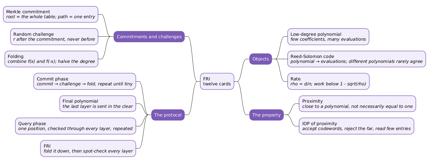
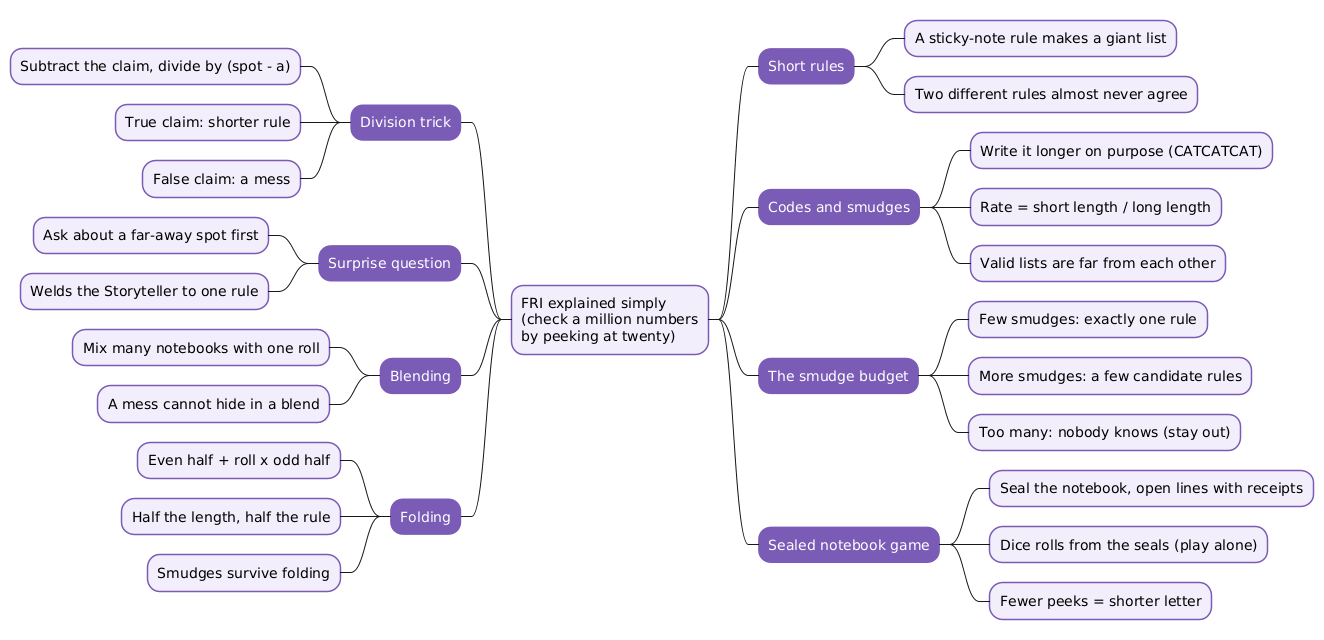
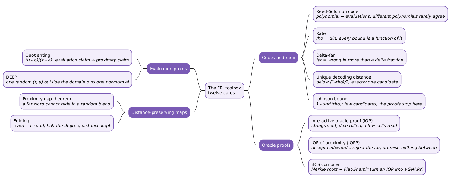
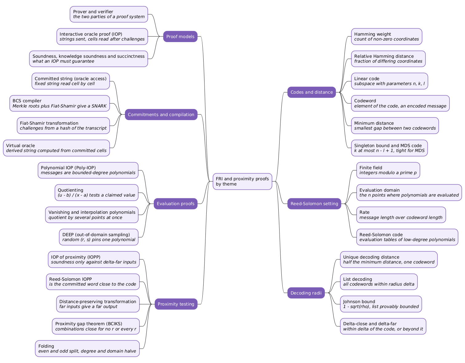
Mindmap of FRI and proximity-proof vocabulary, split into beginner, intermediate and advanced terms including Reed-Solomon code, Johnson bound, IOP of proximity, quotienting and folding

The same thirty terms regrouped by subject rather than by reading order show which entries are one idea seen at several levels: the decoding radii form one cluster, the proof models another, and the compiler tools a third.

Mindmap grouping FRI and proximity-proof vocabulary by theme, with codes and distance, decoding radii, proof models, commitments and compilation, evaluation proofs, and proximity testing branches

Frequently Asked Questions

Q: What is the difference between the Hamming weight and the relative Hamming distance?

The Hamming weight is a property of one vector: the count of its non-zero coordinates. The relative Hamming distance is a property of a pair of vectors: the Hamming weight of their difference, divided by the length. The division is what lets a radius such as $\delta = 1/2$ mean the same thing for a code of length $2^{10}$ and one of length $2^{20}$.

Q: Why is the Johnson bound rather than the unique decoding distance the limit everyone quotes?

Below the unique decoding distance a word has at most one nearby codeword, which is the simplest situation but also the most restrictive: at rate $1/4$ it stops at $3/8$. Below the Johnson bound, $1/2$ at that rate, the number of nearby codewords is no longer one but is still provably bounded, and a bounded list is enough for every argument in the FRI toolbox, from the DEEP union bound to the proximity gap theorem. Above the Johnson bound nothing is proven for structured domains, so it is the largest radius with a guarantee.

Q: How does an IOP of proximity differ from an ordinary IOP?

Two ways. The instance of an IOPP includes a committed string that the verifier can only read cell by cell, whereas an IOP’s instance is given in full. And soundness is relaxed: an IOPP need only reject inputs that are $\delta$-far from the relation, with no requirement on inputs that are close but not in it. The relaxation is forced by the model, since no verifier reading a few cells can detect a single wrong entry.

Q: What does a virtual oracle save, and what does it cost?

It saves a commitment: a derived string such as a quotient or a batched combination is never Merkle-committed, so the proof carries no extra root and the prover does no extra hashing. It costs reads of the underlying strings: opening one cell of a batched word $\sum_j r^j u_j$ requires opening that cell in every $u_j$, each with its own authentication path.

Q: Why does quotienting need DEEP once the proximity parameter exceeds the unique decoding distance?

Quotienting proves that some polynomial in $\mathrm{List}(u, d, \delta)$ takes the claimed value at the query point. Below the unique decoding distance the list has one member, so that polynomial is the committed one. Above it, the list may hold several, and each query could be answered from a different member, so the prover is not bound to a single polynomial. DEEP’s out-of-domain pair $(r, s)$, included in every quotient, singles out one list member with high probability because two distinct low-degree polynomials rarely agree at a random point.

Q: Which property of a Reed-Solomon code makes folding preserve the rate, and why does that matter for the Johnson bound?

A fold halves the degree bound, from $d$ to $d/2$, because the even and odd parts each hold half the coefficients, and it halves the domain, from $L$ to $L^2$, because squaring on a group of roots of unity is two-to-one. The rate $\rho = d/n$ is therefore unchanged. Since the Johnson bound is $1 - \sqrt\rho$, a proximity parameter chosen below it for the original code stays below it for every folded code, so the distance-preservation guarantee applies at every round.

Q: What does “correlated” add to the proximity gap theorem?

Plain proximity would say each $u_j$ is individually within $\delta$ of some codeword, possibly disagreeing with it on different positions for different $j$. Correlated proximity says there is one set $S$ of at least $$(1-\delta)

$positions on which every$u_j$matches its codeword. By linearity, every combination$\sum_j r^j u_j$then matches a codeword on$S$too, for every$r$, which is what produces the all-or-nothing gap in the fraction of good$r$$.

References

Source lecture

ZK Whiteboard Sessions — S2M7: FRI and Proximity Proofs (Part 1), with Dan Boneh
ZK Whiteboard Sessions, the series page

Papers

Eli Ben-Sasson, Iddo Bentov, Yinon Horesh, Michael Riabzev, Fast Reed-Solomon Interactive Oracle Proofs of Proximity, ECCC TR17-134, 2017
Eli Ben-Sasson, Alessandro Chiesa, Nicholas Spooner, Interactive Oracle Proofs, 2016
Eli Ben-Sasson, Lior Goldberg, Swastik Kopparty, Shubhangi Saraf, DEEP-FRI: Sampling Outside the Box Improves Soundness, 2019
Eli Ben-Sasson, Dan Carmon, Yuval Ishai, Swastik Kopparty, Shubhangi Saraf, Proximity Gaps for Reed-Solomon Codes, 2020
Gal Arnon, Alessandro Chiesa, Giacomo Fenzi, Eylon Yogev, STIR: Reed-Solomon Proximity Testing with Fewer Queries, 2024
Ariel Gabizon, Zachary J. Williamson, Oana Ciobotaru, PlonK, 2019
Binyi Chen, Benedikt Bünz, Dan Boneh, Zhenfei Zhang, HyperPlonk, 2022
Alessandro Chiesa, Eylon Yogev, Building Cryptographic Proofs from Hash Functions, 2024

Feel free to contact me on

# zkp # snark # stark # fri # reed-solomon # iop # polynomial-commitment # glossary # key-terms

You might also enjoy

FRI in Twelve Cards — The Definitions to Memorise

FRI Explained Like I'm Ten — How to Check a Million Numbers by Peeking at Twenty

The FRI Toolbox in Twelve Cards — The Definitions to Memorise

FRI and Proximity Proofs, Part 1 — Reed-Solomon Codes, IOPs of Proximity, Quotienting and Folding