The Black-Scholes Model - Pricing Options and Corporate Liabilities
In 1973, Fischer Black and Myron Scholes published The Pricing of Options and Corporate Liabilities in the Journal of Political Economy. The paper gave the first internally consistent formula for the value of a European call option, expressed only in terms of observable quantities and one volatility parameter. Earlier valuation formulas all carried at least one arbitrary parameter, such as an expected return or a discount rate, that nobody could pin down from market data.
The method that removed those parameters is the paper’s central contribution. Black and Scholes construct a portfolio of the stock and the option whose return is riskless over any short interval, then argue that this return must equal the interest rate. That single equilibrium condition produces a differential equation whose solution is the option formula. The same argument then reframes common stock, corporate bonds, and warrants as options on a firm’s assets. This article follows the paper section by section, keeping its original notation.
This article has been made with the help of Claude Code and several custom skills
Notation
The paper prices a call option written on a single share of common stock. The following symbols recur throughout.
| Symbol | Meaning |
|---|---|
| \(x\) | current stock price |
| \(c\) | exercise (striking) price of the option |
| \(t\) | current date |
| \(t^*\) | maturity date, so \(t^* - t\) is the time remaining |
| \(r\) | short-term interest rate, known and constant |
| \(v^2\) | variance rate of the return on the stock, so \(v\) is its volatility |
| \(w(x,t)\) | value of the call option as a function of stock price and time |
| \(u(x,t)\) | value of the corresponding put option |
| \(N(\cdot)\) | cumulative standard normal distribution function |
Subscripts on \(w\) denote partial derivatives: \(w_1\) is the derivative with respect to the first argument \(x\), \(w_2\) the derivative with respect to time \(t\), and \(w_{11}\) the second derivative with respect to \(x\). In modern texts these appear as \(S\), \(K\), \(\sigma\), \(T\), and the Greeks, but the derivation is unchanged.
The valuation problem before 1973
An option is a security giving the right to buy or sell an asset, under fixed conditions, within a set period. An American option can be exercised at any time up to expiration; a European option only at maturity. The call option studied in the paper grants the right to buy one share at the exercise price \(c\).
Qualitative behaviour was already understood.
- When the stock price sits far above the exercise price, the option is almost certain to be exercised, and its value approaches the stock price minus a discount bond with face value \(c\).
- When the stock price sits far below \(c\), exercise is unlikely and the option is nearly worthless.
The two limits are the branches of a single comparison of the stock price against the exercise price, with the near-the-money case in between.
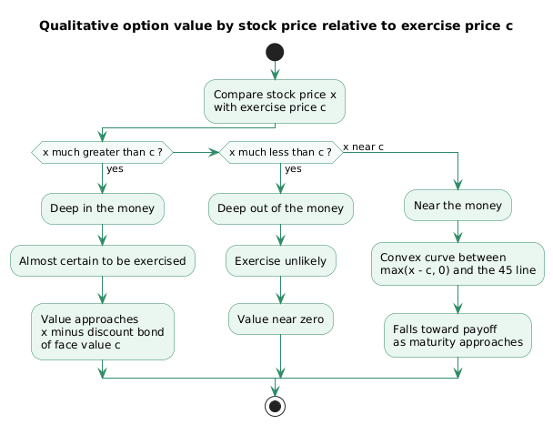
Plotted against the stock price, the option value is a convex curve lying below the 45-degree line and above the payoff \(\max(x - c, 0)\), shifting downward as maturity approaches.
The open problem was a formula. Sprenkle (1961), Ayres (1963), Boness (1964), Samuelson (1965), Baumol, Malkiel and Quandt (1966), and Chen (1970) had all produced expressions of a similar shape. Sprenkle’s value for an option, for instance, takes the form
[\begin{aligned} k x N(b_1) - k^* c\, N(b_2), \end{aligned}]
with \(b_1\) and \(b_2\) built from \(\ln kx/c\) and the variance. The structure anticipates the final answer, but \(k\), the ratio of the expected stock price at maturity to the current price, and \(k^*\), a risk-dependent discount factor, are unknown parameters. Sprenkle tried to estimate them empirically and could not. Samuelson’s formulation likewise carried an expected return \(\alpha\) on the stock and a discount rate \(\beta\) on the warrant, with no equilibrium theory fixing their values.
Black and Scholes drew one idea from Thorp and Kassouf (1967), who fit an empirical warrant formula and used it to build a hedged position long one security and short the other. What Thorp and Kassouf did not pursue is the consequence that the paper turns into a theory: in equilibrium, a fully hedged position must earn the riskless rate. That constraint is what removes the free parameters.
Ideal market conditions
The derivation assumes an idealized market. The assumptions are strong, and the paper states them plainly.
- Constant interest rate. The short-term rate \(r\) is known and constant through time.
- Lognormal stock dynamics. The stock price follows a continuous-time random walk with a variance rate proportional to the square of the price. Prices over any finite interval are lognormally distributed, and the variance rate of the return \(v^2\) is constant.
- No dividends. The stock pays no dividends or other distributions.
- European exercise. The option can be exercised only at maturity.
- No transaction costs. Buying or selling the stock or the option is frictionless.
- Free borrowing. Any fraction of a security’s price can be borrowed to hold it, at the short-term rate.
- No short-selling penalty. A seller who does not own a security can still sell it and settle later at the market price.
Under these conditions the option value depends only on the stock price, on time, and on constants taken as known. That restriction is what makes the hedge below possible.
The hedging argument
Because the option value \(w(x,t)\) moves with the stock and with time only, one can build a position whose value does not depend on the stock price. Hold one share long and sell short a number of options equal to
[\begin{aligned} \frac{1}{w_1(x,t)} \end{aligned}]
options against it. The ratio of the change in option value to the change in stock value, for a small stock move, is \(w_1(x,t)\). A stock move of \(\Delta x\) changes the option by roughly \(w_1 \Delta x\), so short-selling \(1/w_1\) options changes the short side by roughly \(\Delta x\), offsetting the long share. The stock-price risk cancels to first order.
As \(x\) and \(t\) change, the number of options to hold short changes with them, so the hedge must be rebalanced. If the position is adjusted continuously, the first-order approximation becomes exact and the return on the hedged position becomes certain. Robert Merton pointed out this exactness to the authors.
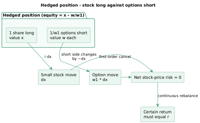
The paper illustrates the position numerically. Take the option maturity curve \(T_2\) of the paper’s figure, with the stock at \(\$15.00\), the option worth \(\$5.00\), and the slope \(w_1 = 1/2\). The hedge is one share long and two options short. The share costs \(\$15.00\), the two options bring in \(\$10.00\), so the equity is \(\$5.00\). If the hedge is left unadjusted, the equity varies slightly with a large stock move: a \(\$5.00\) move in either direction produces about a \(\$0.75\) decline in equity, and the direction of that decline does not depend on the direction of the stock move. Because the shift is independent of direction, the covariance between the hedged return and the stock return is zero, and so is the covariance with the market. The residual risk of an unadjusted hedge is therefore diversifiable, and it vanishes entirely when the hedge is adjusted continuously.
The option pricing differential equation
Write the value of the equity in the hedged position, one share long and \(1/w_1\) options short, as
[\begin{aligned} x - \frac{w}{w_1}. \end{aligned}]
Over a short interval \(\Delta t\), the equity changes by \(\Delta x - \Delta w / w_1\). With the position adjusted continuously, stochastic calculus expands \(\Delta w\) as
[\begin{aligned} \Delta w = w_1 \Delta x + \tfrac{1}{2} w_{11} v^2 x^2 \Delta t + w_2 \Delta t. \end{aligned}]
The first term carries the stock-price randomness; the last two are deterministic over the interval. Substituting this expansion into the equity change, the \(\Delta x\) terms cancel and the change in the equity of the hedged position reduces to
[\begin{aligned} -\left(\tfrac{1}{2} w_{11} v^2 x^2 + w_2\right)\frac{\Delta t}{w_1}. \end{aligned}]
This change is certain, so its return must equal the riskless return on the same equity, which is the equity times \(r \Delta t\). If it did not, speculators would borrow to build the position and arbitrage the difference away. Setting the certain change equal to \((x - w/w_1)\, r \Delta t\) and dropping the common \(\Delta t\) gives the differential equation for the option value:
[\begin{aligned} w_2 = r w - r x w_1 - \tfrac{1}{2} v^2 x^2 w_{11}. \end{aligned}]
The equation is completed by a boundary condition at maturity. At \(t = t^*\) the option is worth its exercise value:
[\begin{aligned}
w(x, t^) &= x - c, \quad x \ge c
w(x, t^) &= 0, \quad x < c.
\end{aligned}]
It is worth tracing why each step appears, because the equation is not guessed but forced by the argument.
- Why the equity is \(x - w/w_1\). The hedge holds one share, worth \(x\), against \(1/w_1\) options sold short, worth \(w\) each, so the short side is a liability of \(w/w_1\). The equity is the net, and writing it this way lets the next step track a single quantity through the interval.
- Why the expansion of \(\Delta w\) has three terms. The option value is a function of two variables, so its change comes from the stock move and the passage of time. Ordinary calculus would keep only \(w_1 \Delta x\) and \(w_2 \Delta t\), but the stock is a diffusion whose squared move \((\Delta x)^2\) is of order \(\Delta t\) rather than negligible. Stochastic calculus therefore retains the second-order term \(\tfrac{1}{2} w_{11} v^2 x^2 \Delta t\), which carries the volatility into the equation. This extra term is the reason volatility ends up as the formula’s central input.
- Why the \(\Delta x\) terms cancel. The number of options shorted was chosen as exactly \(1/w_1\) so that the option’s first-order response \(w_1 \Delta x\) is scaled back to \(\Delta x\) and subtracted from the share’s \(\Delta x\). The random term disappears by construction, leaving only the deterministic pieces. This cancellation is the whole point of the hedge.
- Why the result must equal \(r\,\Delta t\) per unit of equity. Once the change is certain, the position is riskless over the interval. Two riskless investments cannot offer different returns without inviting unbounded arbitrage, so the hedged equity must grow at the interest rate. Equating the certain change to the riskless return and cancelling the common \(\Delta t\) leaves a relation among \(w\) and its derivatives, which is the differential equation.
- Why a boundary condition is needed. The equation constrains how \(w\) changes but not its overall level; many functions satisfy it. Fixing the value at maturity, where the option is simply worth \(\max(x - c, 0)\), selects the one solution that is an actual option price.
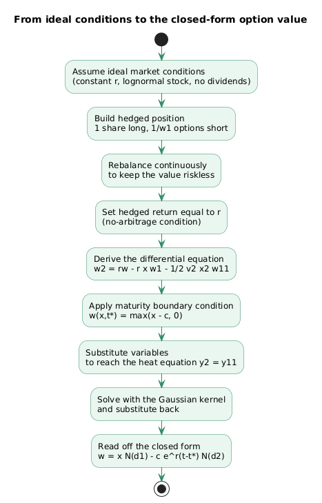
Only one function \(w(x,t)\) satisfies the equation subject to this condition, and that function is the option formula. The derivation is summarized below.
Solving the equation
A change of variables converts the option equation into the heat-transfer equation of physics. Under the substitution the paper uses, the differential equation becomes \(y_2 = y_{11}\), the standard diffusion equation, and the maturity condition becomes an initial condition on \(y\). The solution of the heat equation is a known Gaussian integral, given in Churchill’s Fourier Series and Boundary Value Problems. Substituting back and simplifying yields the closed form:
[\begin{aligned} w(x,t) = x N(d_1) - c\, e^{r(t - t^*)} N(d_2), \end{aligned}]
with
[\begin{aligned} d_1 = \frac{\ln x/c + \left(r + \tfrac{1}{2} v^2\right)(t^* - t)}{v \sqrt{t^* - t}}, \end{aligned}]
[\begin{aligned} d_2 = \frac{\ln x/c + \left(r - \tfrac{1}{2} v^2\right)(t^* - t)}{v \sqrt{t^* - t}} = d_1 - v \sqrt{t^* - t}. \end{aligned}]
Here \(e^{r(t - t^*)}\) is a discount factor, since \(t - t^*\) is negative, and \(N(\cdot)\) is the cumulative normal distribution. The first term \(x N(d_1)\) is the present value of receiving the stock if the option finishes in the money; the second term \(c\, e^{r(t-t^*)} N(d_2)\) is the present value of paying the exercise price, weighted by the risk-neutral probability \(N(d_2)\) that exercise occurs.
Two features of the formula deserve emphasis.
- No expected return. The expected return on the stock does not appear anywhere in the formula. Two investors who disagree about how fast the stock will rise still agree on the option’s value, provided they agree on the volatility. The expected return is already reflected in the current stock price, and the hedging argument prices the option relative to that stock price, not relative to a forecast.
- Maturity enters through \(r\) and \(v^2\) only. The time to maturity \(t^* - t\) appears only multiplied by the interest rate or the variance rate. Increasing maturity has the same effect as an equal percentage increase in both \(r\) and \(v^2\). Merton (1973) showed that the value rises continuously as any of \(t^* - t\), \(r\), or \(v^2\) increases, approaching the stock price as an upper bound.
The partial derivative of the formula, the hedge ratio itself, simplifies to
[\begin{aligned} w_1(x,t) = N(d_1). \end{aligned}]
This is the modern delta: the number of shares to hold against one option, or the slope of the value curve. The factor \(x w_1 / w\) is always greater than one. This follows from the formula itself: since \(x w_1 = x N(d_1)\) and \(w = x N(d_1) - c\, e^{r(t-t^*)} N(d_2)\), their difference is \(x w_1 - w = c\, e^{r(t-t^*)} N(d_2)\), which is strictly positive because the exercise price, the discount factor, and the probability \(N(d_2)\) are all positive. So \(x w_1\) exceeds \(w\), and the ratio exceeds one. The economic reason is leverage: holding the call is like owning \(N(d_1)\) shares while having borrowed part of the cost, so the amount actually put in is smaller than the shares it controls, and a given stock move is a larger percentage move on that smaller base. This ratio is the amplification from the stock’s return to the option’s return, since the dominant random part of the option move is \(\Delta w \approx w_1 \Delta x\), which in percentage terms reads \(\Delta w / w \approx (x w_1 / w)(\Delta x / x)\). The option’s percentage return is the stock’s percentage return magnified by \(x w_1 / w\), so its volatility is larger by that same factor. The option is therefore always more volatile than the underlying stock, which is why a hedge of options against stock is needed in the first place.
An alternative derivation through the CAPM
The same differential equation follows from the capital asset pricing model, and that route is worth stating because it clarifies how an uncertain future payoff is discounted to the present. The CAPM says an asset’s expected return above the riskless rate is proportional to its beta, the covariance of its return with the market return divided by the variance of the market return.
From the stochastic expansion of \(\Delta w\), the covariance of the option return with the market equals \(x w_1 / w\) times the covariance of the stock return with the market. The option and stock betas therefore satisfy
[\begin{aligned} \beta_w = \frac{x w_1}{w}\, \beta_x. \end{aligned}]
The factor \(x w_1 / w\) is the elasticity of the option price with respect to the stock price, the ratio of the percentage change in the option to the percentage change in the stock. Writing the expected returns on the stock and the option through the CAPM, expanding \(\Delta w\) with stochastic calculus, and taking expectations, the terms that carry the market risk premium and the stock beta cancel exactly. What remains is
[\begin{aligned} w_2 = r w - r x w_1 - \tfrac{1}{2} v^2 x^2 w_{11}, \end{aligned}]
the same equation as before. The hedging argument and the equilibrium-pricing argument lead to one place. The cancellation of the risk terms is the CAPM statement of the same fact the hedge shows directly: the option’s systematic risk is entirely inherited from the stock, so no independent risk premium survives.
Put options and put-call parity
A European put option, the right to sell at \(c\), obeys the same differential equation with a mirrored boundary condition: at maturity the put is worth \(c - x\) when \(x < c\) and zero otherwise. Rather than resolve the equation, the paper notes that the difference between a call and a put on the same stock must itself satisfy the differential equation, with the boundary condition \(w(x,t^*) - u(x,t^*) = x - c\). The solution of that difference is
[\begin{aligned} w(x,t) - u(x,t) = x - c\, e^{r(t - t^*)}. \end{aligned}]
This is put-call parity. Holding a call and writing a put gives the same payoff as buying the stock on margin, borrowing \(c\, e^{r(t-t^*)}\) toward its price. Substituting the call formula and using \(1 - N(d) = N(-d)\) gives the put directly:
[\begin{aligned} u(x,t) = -x N(-d_1) + c\, e^{r(t - t^*)} N(-d_2). \end{aligned}]
The parity relation was first noted by Stoll (1969), though the paper observes that it holds only for European options. Merton (1973) showed that an American put is worth more than a European put, because early exercise can be advantageous when the stock price falls near zero: exercising then collects the exercise price sooner and earns interest on it. No closed formula for the American put value was known at the time of writing.
Corporate liabilities as options
The reach of the paper comes from a reinterpretation. Almost every corporate liability can be read as an option on the firm’s assets, so the same formula prices them.
Consider a company whose only assets are shares of a second company, financed by common stock and a single issue of pure discount bonds with face value \(c\) maturing in ten years, with no dividends allowed until the bonds are paid. At maturity the firm sells its assets, pays the bondholders if it can, and hands the rest to the stockholders. The stockholders hold a call option on the firm’s assets: they own the assets but have granted the bondholders the right to take them back for \(c\). Whichever party has the claim, the stock is worth \(w(x,t)\) from the option formula, where \(x\) is now the total asset value and \(v^2\) the variance rate of the assets, and the bonds are worth \(x - w(x,t)\).
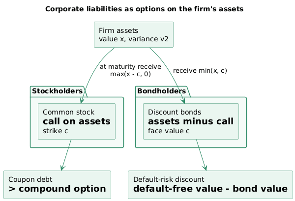
That decomposition carries several consequences the paper draws out.
- A discount for default risk. Subtracting the option value of the bonds from their default-free value gives the discount that default risk imposes on corporate debt, computed rather than assumed.
- Capital structure and the value of debt. The Modigliani-Miller result reappears: the total firm value is the sum of stock and bonds and does not depend on how the two are split. Increasing leverage while holding total value fixed raises the default probability and lowers the market value of each bond, because the face value \(c\) rises faster than the market value \(x - w(x,t)\).
- Dividends transfer value to stockholders. Because a dividend reduces the assets backing the bonds, a larger dividend always favours the stockholders over the bondholders, which is why bond indentures restrict dividend policy.
- Coupon debt as a compound option. With coupon bonds rather than discount bonds, the common stock becomes a compound option, an option on an option, and so on. Each interest payment buys the stockholders the right to make the next payment and keep the firm; the final payment buys the firm outright from the bondholders.
Warrants extend the same idea, with adjustments for their multi-year life, unadjusted exercise prices, and the dilution that exercising many warrants causes. Convertible bonds, callable bonds, and sinking-fund provisions each add a further option to the package. The paper is candid that these more complicated instruments break an assumption of the formula: the variance rate of an option’s return is not constant, so equation (13) cannot value an option on an option exactly, though the same reasoning supports a numerical solution.
Empirical tests
Black and Scholes tested the formula against a large body of over-the-counter call-option prices in a companion study, The Valuation of Option Contracts and a Test of Market Efficiency. The results show systematic deviations.
- Option buyers consistently paid more than the formula predicted, while option writers received roughly the predicted level, a gap attributable to the large transaction costs that buyers effectively bear in that market.
- The spread between the price buyers paid and the formula value was wider for options on low-variance stocks than on high-variance stocks, which means the market underweighted differences in variance when pricing options. Given the transaction costs, the authors note that this misvaluation did not by itself offer a profit opportunity to a speculator.
Conclusion
The 1973 paper solved the option valuation problem by changing the question. Instead of forecasting a stock’s expected return and discounting a payoff, it built a continuously rebalanced hedge whose return is riskless, set that return equal to the interest rate, and read off a differential equation. The equation has one solution meeting the maturity payoff, and that solution is the call formula \(w(x,t) = x N(d_1) - c\, e^{r(t-t^*)} N(d_2)\). The expected return on the stock never enters, which is why two investors with different forecasts still agree on the option’s price.
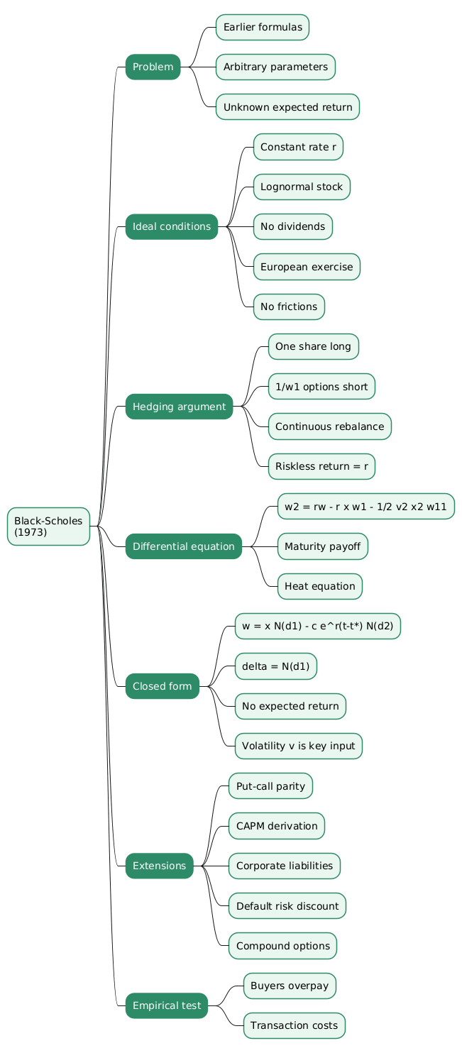
The volatility \(v^2\) is the only input not directly observable, and it became the quantity option markets now trade around. The second half of the paper showed that common stock, corporate bonds, warrants, and convertibles are options on a firm’s assets, so the formula prices corporate liabilities and quantifies the discount that default risk applies to debt. The empirical companion study found the model close to writer-side prices with buyer-side deviations traceable to transaction costs. The mindmap below collects the paper’s structure.
Annex
Key Terms
| Term | Definition |
|---|---|
| Call option | A security giving the right, but not the obligation, to buy one share at the exercise price \(c\) within a set period. |
| European option | An option that can be exercised only on the maturity date \(t^*\), not before, which the closed-form formula assumes. |
| Exercise price | The fixed price \(c\) paid for the share when the option is exercised, also called the striking price. |
| Hedged position | One share held long against \(1/w_1\) options sold short, constructed so its value does not depend on the stock price to first order. |
| Hedge ratio (delta) | The number of shares to hold against one option, equal to \(w_1 = N(d_1)\), the slope of the option value curve. |
| Variance rate | The quantity \(v^2\), the limiting variance of the stock’s return per unit time, whose square root \(v\) is the volatility and the formula’s only non-observable input. |
| Option pricing equation | The differential equation \(w_2 = r w - r x w_1 - \tfrac{1}{2} v^2 x^2 w_{11}\) that the option value must satisfy under the ideal conditions. |
| Put-call parity | The relation \(w - u = x - c\, e^{r(t-t^*)}\) linking the values of a European call and put on the same stock. |
| Elasticity | The factor \(x w_1 / w\), the ratio of the percentage change in the option price to the percentage change in the stock price, always greater than one. |
| Compound option | An option whose underlying is itself an option, the reading of common stock when a firm carries coupon debt rather than pure discount bonds. |
| Option writer | The party who sells (writes) the option and takes the short side, receiving the premium and bearing the obligation to deliver if the holder exercises. |
| Capital asset pricing model (CAPM) | The equilibrium model in which an asset’s expected excess return is proportional to its beta, used in the paper as a second route to the same option pricing equation. |
| Heat equation | The diffusion equation \(y_2 = y_{11}\) of physics, into which a change of variables converts the option pricing equation so that its known Gaussian solution can be borrowed. |
| Deep in the money | The regime where the stock price sits far above the exercise price \(c\), so exercise is almost certain and the call value approaches the stock price minus a discount bond of face value \(c\). |
| Stochastic calculus | The calculus of quantities driven by continuous random motion, which expands the option’s change with an extra second-order term \(\tfrac{1}{2} w_{11} v^2 x^2 \Delta t\) because a diffusion’s squared move is of order \(\Delta t\) rather than negligible. |
Frequently Asked Questions
Q: Why does the expected return on the stock not appear in the formula?
The valuation is built from a hedged position that is riskless over each short interval, so its return must equal the interest rate regardless of anyone’s forecast for the stock. The option is priced relative to the current stock price, which already embeds the market’s view of the expected return. Two investors who disagree about how fast the stock will rise, but agree on its volatility, therefore compute the same option value. The expected return does affect how fast the option price rises over time, because that price moves with the stock, but it does not enter the level of the formula.
Q: What role does the volatility \(v^2\) play, and why is it special among the inputs?
The variance rate \(v^2\) is the only input to the formula that is not directly observable in the market. The stock price, exercise price, interest rate, and time to maturity are all quoted or contractual, but volatility must be estimated. It governs the width of the distribution of possible future stock prices, and a higher volatility raises the option value because it increases the chance of a large favourable move while the downside is capped at the premium. Because it is the single free quantity, option markets came to quote and trade implied volatility directly.
Q: How is the hedged position constructed, and why must it be rebalanced?
The position holds one share long and sells short \(1/w_1\) options, where \(w_1\) is the slope of the option value with respect to the stock price. A small stock move changes the long share and the short options by offsetting amounts, so the stock-price risk cancels to first order. The slope \(w_1\) itself depends on the stock price and on time, so as either changes the correct number of options to hold short changes too. Keeping the hedge riskless therefore requires continuous rebalancing; if the position is left unadjusted, a residual risk appears, but it is diversifiable and its covariance with the market is zero.
Q: In what sense is a company’s common stock an option?
For a firm financed by stock and a single issue of discount bonds with face value \(c\), the stockholders receive the firm’s assets minus \(c\) at maturity if that difference is positive, and nothing otherwise. That payoff is exactly the payoff of a call option on the firm’s assets with exercise price \(c\). The stockholders effectively own the assets but have sold the bondholders the right to reclaim them for \(c\). Applying the option formula with \(x\) set to the total asset value and \(v^2\) to the variance of the assets prices the stock, and the bonds are worth the assets minus that option value.
Q: How does the CAPM derivation reach the same differential equation as the hedging argument?
The capital asset pricing model expresses each asset’s expected excess return through its beta. Using the stochastic expansion of the option’s change, the option’s beta equals its elasticity \(x w_1 / w\) times the stock’s beta. Writing the expected returns on the stock and option through the CAPM, expanding the option change with stochastic calculus, and taking expectations, the terms carrying the market risk premium and the stock’s beta cancel. What remains is the same option pricing equation. Both routes encode one fact: the option’s systematic risk is entirely inherited from the stock, so no separate risk premium survives, which is why the expected return drops out.
Q: Why does the formula apply to a European call and an American call alike but not to an American put?
Merton showed that the value of a live call always exceeds its immediate exercise value \(x - c\), so a rational holder of an American call on a non-dividend-paying stock never exercises early. Early exercise is never optimal, and the American call is worth the same as the European call the formula prices. A put is different: if the stock price falls near zero, exercising the put early collects the exercise price sooner and earns interest on it, which can be worth more than waiting. Early exercise can therefore be optimal for an American put, its value exceeds the European put, and no closed-form formula for it was known when the paper was written.
References
- Black, Fischer, and Myron Scholes. “The Pricing of Options and Corporate Liabilities.” Journal of Political Economy 81, no. 3 (1973): 637-654.
- Black, Fischer, and Myron Scholes. “The Valuation of Option Contracts and a Test of Market Efficiency.” Journal of Finance 27, no. 2 (1972): 399-417.
- Merton, Robert C. “Theory of Rational Option Pricing.” Bell Journal of Economics and Management Science 4, no. 1 (1973): 141-183.
- Sprenkle, Case. “Warrant Prices as Indications of Expectations.” Yale Economic Essays 1 (1961): 179-232.
- Thorp, Edward O., and Sheen T. Kassouf. Beat the Market. New York: Random House, 1967.
- Samuelson, Paul A. “Rational Theory of Warrant Pricing.” Industrial Management Review 6 (1965): 13-31.
- Modigliani, Franco, and Merton H. Miller. “The Cost of Capital, Corporation Finance and the Theory of Investment.” American Economic Review 48 (1958): 261-297.
- Stoll, Hans R. “The Relationship Between Put and Call Option Prices.” Journal of Finance 24 (1969): 802-824.
- Churchill, R. V. Fourier Series and Boundary Value Problems. 2nd ed. New York: McGraw-Hill, 1963.
- Claude Code
Related articles
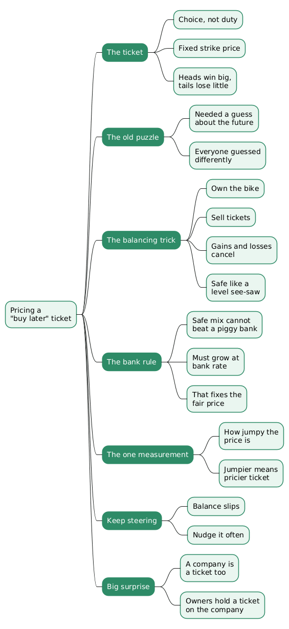
- The Black-Scholes Model for Curious Kids — Pricing a Ticket to Buy Later
- Traditional Futures vs. Perpetual Futures: A Technical Comparison
You might also enjoy