Recurrent Neural Networks (RNNs) - Overview
Artificial neural networks (ANNs) have evolved into a diverse family of architectures designed to process various types of data and tasks. Among these, Recurrent Neural Networks (RNNs) are known for their ability to model sequential and temporal dependencies, making them fundamental in natural language processing (NLP), speech recognition, and time-series prediction.
This article provides a technical overview of RNNs, explains their internal mechanisms, and compares them with other major architectures—Perceptrons, Convolutional Neural Networks (CNNs), and Transformers.
[TOC]
What is an RNN?
An RNN is a neural network designed to recognize patterns in sequences of data, such as text, time series, speech, or video. Unlike traditional feedforward neural networks, RNNs have loops within their architecture. These loops allow information to persist, meaning the network has a “memory” of previous inputs, making it well-suited to sequential tasks.
At each time step, the RNN takes an input and combines it with the “hidden state” (the memory from previous steps) to produce an output and an updated hidden state. This recurrent mechanism enables the network to model temporal dynamics.
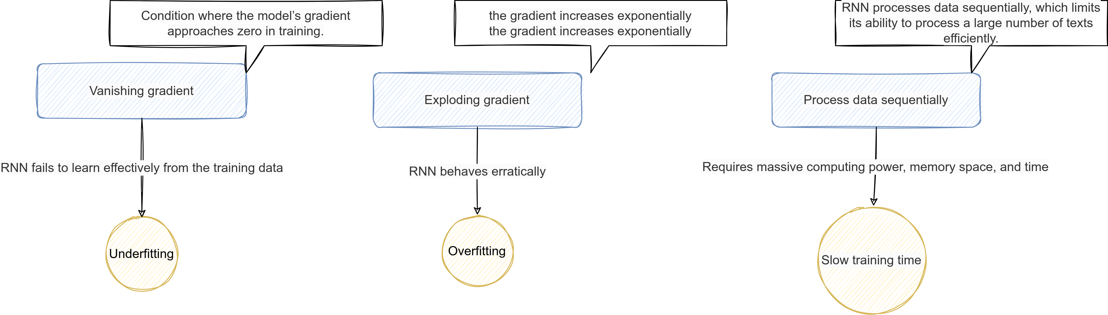
Key characteristics of RNNs and limitation:
- Sequential Processing: Data is processed step-by-step, respecting order.
- Parameter Sharing: The same weights are reused at every time step.
- Memory: Past information can influence future outputs.
However, standard RNNs face challenges like vanishing and exploding gradients, which make it difficult for them to capture long-term dependencies.
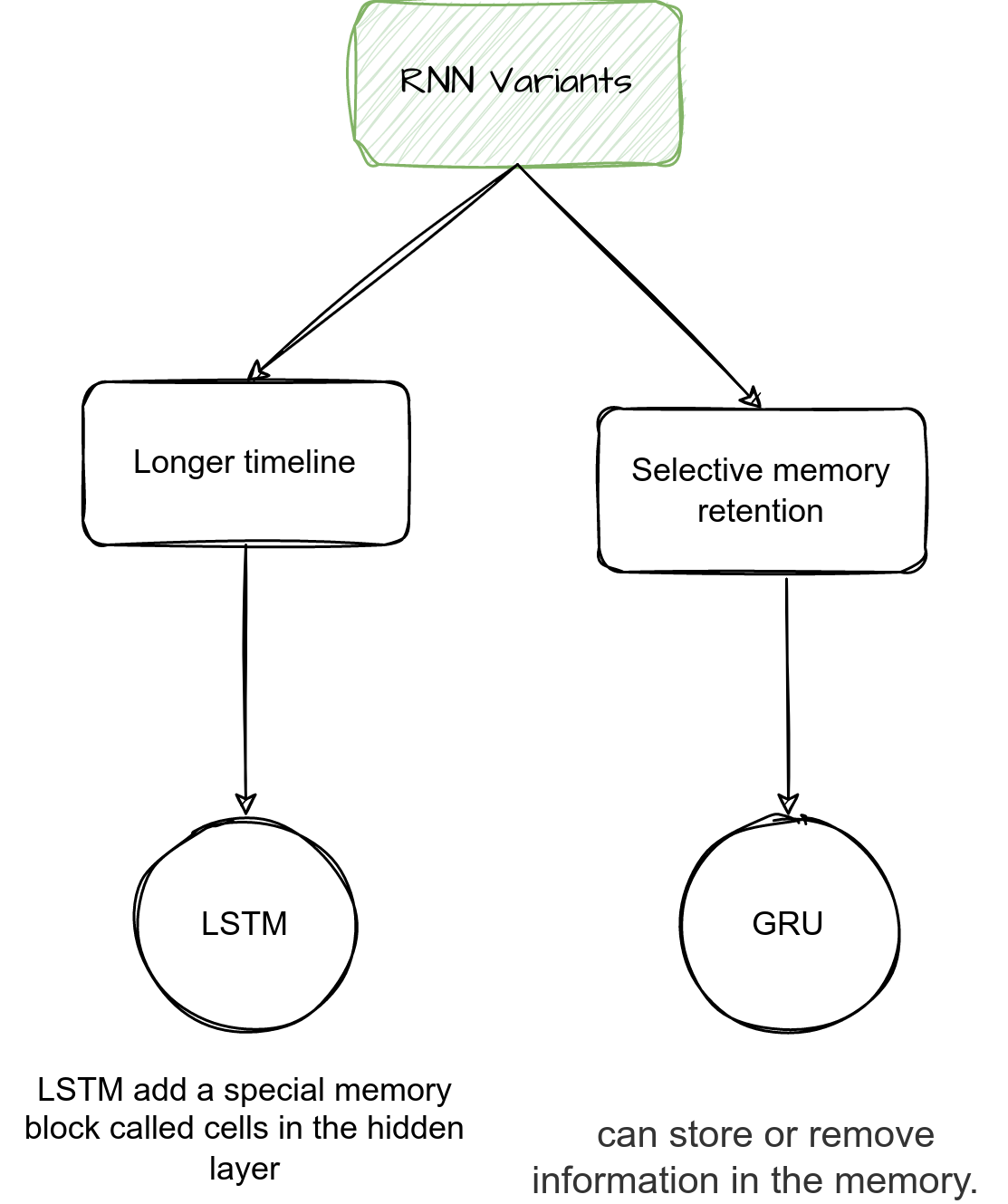
Variants like Long Short-Term Memory (LSTM) and Gated Recurrent Units (GRU) were developed to address these issues.
Schema
Mathematical Formulation
Hidden state update
Given a sequence of inputs x1,x2,…,xT, an RNN computes:
[\begin{aligned} h_t=f(W_{xh}x_t+W_{hh}h_{t−1}+bh) \end{aligned}]
Where:
htis the hidden state at time t,W_xh,W_hh,W_hyare weight matrices,fis an activation function (typically tanh or ReLU).
Output computation: \(\begin{aligned} y_t =g(W_{hy}ht+by) \end{aligned}\)
Where:
- y_t: raw output (logits) at time t
[y_t \in \mathbb{R}^{d_y}]
- W_hy: hidden-to-output weights.
[W_{hy} \in \mathbb{R}^{d_y \times d_h}]
by: output bias.g: If used for classification,ytis typically passed to a Softmax function.
Note: d represents the dimension (size) of a vector space. It tells you how many components the vector has.
Activation Functions and Loss in RNNs
ReLU (Rectified Linear Unit)
Introduces non-linearity in the network, allowing it to learn complex patterns. ReLU outputs zero for negative inputs and passes positive inputs unchanged.
- Usage in RNNs: Often applied in the hidden layers or hidden state transformations to help mitigate the vanishing gradient problem and speed up training. While traditional RNNs use tanh or sigmoid, ReLU is sometimes preferred in modern variants for efficiency.
Softmax
Converts the raw output of the network into a probability distribution over multiple classes. Each value is between 0 and 1, and the sum across all classes equals 1.
This is used at the output layer of RNNs that perform classification or sequence prediction (e.g., predicting the next word). \(\hat{y}_{t,i} = \text{Softmax}(y_t)_i = \frac{e^{y_{t,i}}}{\sum_{j=1}^{K} e^{y_{t,j}}}\) Where:
- y_{t,i]} the logit (raw score) for class i.
- y^_t,i predicted probability for class i.
-
The denominator ensures all probabilities sum to 1.
- Usage in RNNs: Typically applied at the output layer when predicting categorical sequences, such as words in language modeling or discrete classes in classification tasks.
Cross-Entropy Loss
Measures the difference between the predicted probability distribution (from Softmax) and the true labels. It penalizes incorrect predictions more heavily the more confident the network is in them. \(\begin{aligned} \mathcal{L} = - \sum_{i=1}^{K} y_i \log(\hat{y}_i) \end{aligned}\) Where:
yiis the true one-hot label,-
y^iis the predicted probability from Softmax. - Usage in RNNs: Used as the loss function during training, guiding the network to adjust weights so that the predicted probabilities align with the actual sequence labels. This is essential for tasks like language modeling, sequence classification, and speech recognition.
Types of RNNs
To address these limitations, specialized architectures were developed:
- Long Short-Term Memory (LSTM): Introduces gates (input, forget, output) to control information flow.
-
Gated Recurrent Unit (GRU): Simplifies LSTM structure while retaining similar performance.
- Bidirectional recurrent neural networks (BRRNs)
- Encoder-decoder RNN
| Type | Description | Strengths | Weaknesses |
|---|---|---|---|
| Standard RNN | Basic RNN architecture with feedback loops for memory over sequences. | Simple, lightweight, easy to implement. | Struggles with long-term dependencies (vanishing/exploding gradients). |
| Bidirectional RNN (BRNN) | RNN that processes the sequence in both forward and backward directions and combines the information. | Can access both past and future context, improving accuracy in many tasks. | Doubles the computational load; not suitable for real-time applications. |
| Long Short-Term Memory (LSTM) | RNN variant with special gates (input, forget, output) to manage memory and handle long-term dependencies. | Excellent at learning long-term relationships; widely used in NLP and time series. | More complex and computationally expensive than standard RNNs. |
| Gated Recurrent Unit (GRU) | A simplified version of LSTM with fewer gates (update and reset gates). | Faster to train, fewer parameters; good balance between performance and complexity. | May be slightly less expressive than LSTM for very complex patterns. |
| Encoder-Decoder RNN | A two-part architecture: encoder summarizes input into a fixed vector; decoder generates output from that vector (common in seq2seq tasks). | Great for variable-length input/output tasks like translation, summarization. | Performance drops for very long sequences without attention mechanisms. The fixed-length context vector can be a bottleneck, especially for long input sequences. |
Schema
Comparison with Other Neural Architectures
Summary tab
| Aspect | Perceptron | CNN | RNN | Transformer |
|---|---|---|---|---|
| Data Type | Static, non-sequential | Spatial data (images/video) | Sequential (text, time series) | Sequential (text, audio) |
| Architecture | Single-layer linear model | Hierarchical convolutional filters | Recurrent hidden state | Attention-based encoder-decoder |
| Memory / Context | None | Local (spatial) | Temporal (via hidden state) | Global (via self-attention) |
| Parallelization | High | High | Low (sequential dependency) | Very high |
| Gradient Issues | N/A | Mild | Vanishing/exploding gradients | Minimal |
| Interpretability | High | Moderate | Moderate | Moderate to Low |
| Typical Applications | Classification, regression | Vision, feature extraction | NLP, speech, time-series | NLP, multimodal tasks, generative models |
RNN vs. Perceptron
- Perceptron: The simplest form of a neural network, consisting of a single layer of weights followed by an activation function. It processes one input at a time and has no concept of sequence or memory.
- RNN: Extends the perceptron by introducing the notion of time and sequence. It has feedback connections (recurrent loops) that allow it to maintain a state across inputs.
Summary: A Perceptron handles static data points independently; an RNN handles sequences with context from past data.
RNN vs. CNN
- CNN: Primarily designed for spatial data like images. It uses convolutional layers to detect local patterns (e.g., edges in an image) and pooling layers to downsample feature maps.
- RNN: Primarily designed for temporal data, where the sequence and timing of inputs are critical.
While CNNs are highly effective for visual tasks, they are less natural fits for time-series or language modeling where RNNs shine. However, CNNs have been adapted for sequential data too (e.g., Temporal Convolutional Networks, or TCNs), offering competitive or even superior performance in some cases because of their ability to capture dependencies without the vanishing gradient problem.
Summary: CNNs excel in spatial pattern recognition; RNNs excel in temporal pattern recognition.
More information in my article on CNN: Convolutional Neural Networks - Overview
RNN vs. Transformer
- Transformer: A more recent architecture that has largely supplanted RNNs in fields like NLP. Transformers rely entirely on attention mechanisms instead of recurrence to model dependencies, allowing for greater parallelization and the ability to capture long-range relationships effectively.
- RNN: Processes sequences step-by-step, making it inherently sequential and harder to parallelize.
Transformers, through mechanisms like self-attention, can look at all parts of the sequence at once, leading to faster training and better modeling of long-range dependencies. This is why models like GPT, BERT, and T5 are built on Transformer architectures rather than RNNs.
Transformers can capture long-range dependencies much more effectively, are easier to parallelize and perform better on tasks such as NLP, speech recognition and time-series forecasting.
Summary
Transformers outperform RNNs on long sequences, offering more efficient training and better results, especially in large-scale tasks.
- Computation: Transformers allow parallel processing of sequences, while RNNs process them sequentially.
- Long-Term Dependencies: Transformers capture these efficiently through attention weights, whereas RNNs struggle with long-range dependencies.
- Scalability: Transformers scale better with data and compute resources.
- Performance: Transformers now dominate NLP and sequence modeling tasks (e.g., GPT, BERT), effectively replacing RNNs in most applications.
See also my article on the Transformer architecture
Conclusion
Recurrent Neural Networks revolutionized sequential data modeling by introducing the concept of temporal memory.
However, they are gradually being supplanted by attention-based architectures that offer better scalability and parallelization.
However, RNNs still hold practical value when:
- Data is relatively short or streaming in nature.
- Computational resources are limited.
- Low latency and smaller model size are priorities.
They remain effective in certain real-time systems and embedded applications, such as sensor analysis, gesture recognition, and low-power NLP inference.
Reference
- Stanford - Recurrent Neural Networks cheatsheet
- AWS - What is RNN (Recurrent Neural Network)?
- ChatGPT with the input “Write me an article about RNN, include a comparison with CNN, Perceptron and transformer.”, “Add a paragraph to explain the role of relu softmax cross-entropy in RNN”